4. Data Analysis and Collaboration using Hydroshare Workflows
Overview
Questions
- How do users discover and join an existing research group in HydroShare?
- How do users access existing resources and scientific workflows in a group?
- How can users use an existing workflow to carry out data analysis?
Objectives
- Allow the audience some experience using science gateways and existing workflows for data analysis in a collaborative environment
In the following sections, examples are provided to gain hands-on experience discovering groups and resources of interest, joining a collaborative environment, and performing analysis on data who’s results can be written back to HydroShare to share with others in the group.
More specifically, users will learn the following:
- How to discover and join an existing group of interest
- How to navigate the groups landing page and access its resources
- How to use an existing workflow to carry out some data analysis using a JupyterHub workflow
- How to write results back into HydroShare as a new resource to share your analysis with others.
Before starting this activity please be sure to be logged into HydroShare.
Discovering/Finding a HydroShare Group
HydroShare provides a simple search functionality to help users discover and find groups within its site. Use the Collaborate tab at the top of the HydroShare page.
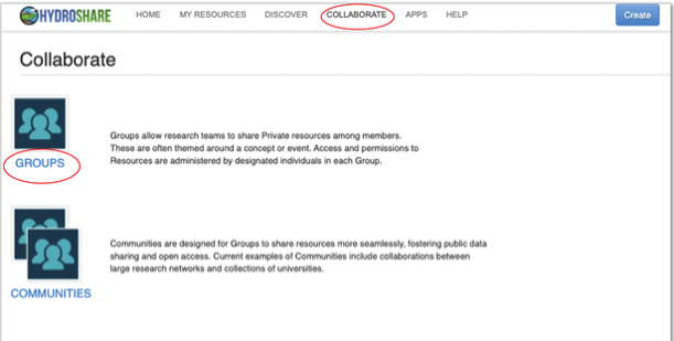
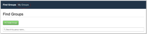
The “Find Groups” page can then be used to find a listing of discoverable and public groups available. Using the search function users can enter keywords which may be associated with group names, purpose, descriptions and other keywords indexed by the group owner.
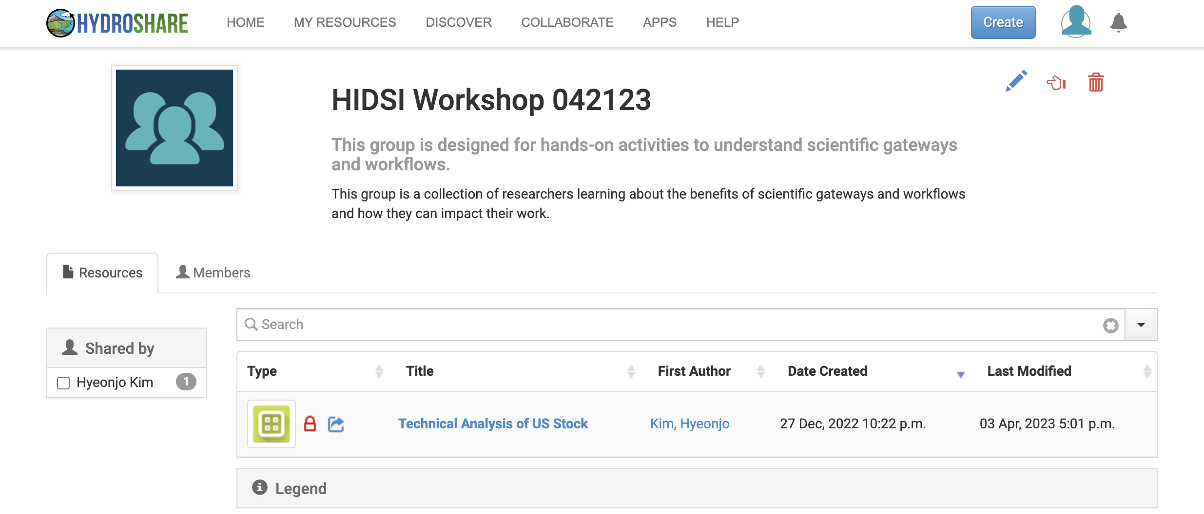
Discover the HIDSI Workshop Group
- Use HydroShare’s search functionality to find the HydroShare group named, “HIDSI Workshop 042123”.
Click on the title of any listed group to view the groups landing page. Members of public groups can be seen by searching users while the members of a discoverable group can not be seen. Either way users can request group membership.
Joining a Group
Once a group of interest is found, users can request access by clicking the “Ask to join” button. If the owner of the group has not set the “auto accept” option for new requests, users may experience a wait time until their request is processed. Otherwise, access may be granted almost immediately.
Join the HIDSI Workshop Group
- Once the “HIDSI Workshop 042123” group is found, request access by clicking, “Ask to join”.
About Groups
A groups landing page will provide some information about the group such as the groups title, purpose and description of the group. From the landing page, users will be able to see all resources shared with the group as well as all members of the group. It should be noted that resources within the group are not owned by all members. While they are shared, ownership is retained by the individual user which created the resource.
Exercise: Using Resources and Workflows Within a Group to Collaborate On Data Analysis
For this exercise, attendees who have joined the HIDSI group will use an existing shared resource containing both data and a Jupyter Notebook workflow to perform some visualization and data analysis. The purpose of this exercise is to:
- Demonstrate how a gateway can provide a collaborative environment
- Demonstrate how data workflows can ease the researchers burden of programming certain computational tasks from scratch.
- Exemplify the usefulness of gateways and workflows in the reproducibility of scientific results.
HydroShare supports various web apps which workflows and models can be built in. Typically, most hydrological modeling and data analysis is done on a personal computer or on some centralized computing system. A user’s knowledge of such centralized computing system could all be barriers to the user’s research. Some examples could be:
- Knowledge about high-performance computing systems
- Capacity of a local computer
- Compatability and dependency requirements for installation on local computers, and
- Time taken to get local model installations properly configured and validated
By providing and supporting web apps such as JupyterHub and its Jupyter Notebook functionality, HydroShare enables a more flexible environment for model execution and data analysis. This gives users a preconfigured environment free of worry about cyberinfrastructure and dependencies thus lowering the forementioned barriers to research.
A Jupyter notebook contains live code, equations, visualization, and explanatory text. They can be used to implement scientific workflows and other computational tasks. HydroShare users can either create and share their own workflows using Jupyter notebooks or discover and use existing workflows implemented as Jupyter notebooks.
Jupyter Notebook functionality within HydroShare:
- Notebooks can be launched from HydroShare
- Notebooks can access the contents of HydroShare resources
- Notebooks can save results back into HydroShare
- Ease of Use For the User
The code within a Jupyter notebook can execute operating and language specific commands within the hosting environment. This provides users with access to the hosting environment’s computational capabilities while eliminating the need for users to install and configure software.
While this does not relieve the user from needing to learn the programming language, operating system commands, or commands associated with the program being used for analysis, it does remove the need for users to install and have the capacity to run these programs locally.
About the Following Exercise
For this exercise attendees will be performing some visualization and data analysis on the stock performance in the United States. They will use an existing workflow to perform some common computational tasks on the type of data provided using several trading indicators of technical analysis. Attendees will then perform further analysis on the data and write their results back to HydroShare as a new separate resource. This resource can then be shared with a group for further scientific collaboration.
- The Data
The data used in this workshop is daily stock data from Yahoo Finance. Yahoo Finance is an online platform that provides financial news and market data, including historical stock quotes and financial reports.
Workflow for Technical Analysis of U.S. Stock
The Jupyter Notebook extracts daily stock data from Yahoo Finance and illustrates the technical analysis of US stocks.
Investment Disclaimer
The information contained on this website and the resources available for this workshop through this website are not intended as, and shall not be understood or construed as, financial advice.
Preparation Step: Accessing the JupyterHub Notebook
- Once on the group landing page, select the resource titled “Technical Analysis of US Stock”
- Click “Open with” at the top right.
- Choose CUAHSI JupyterHub as the webapp.
- Agree to the terms of use and click “Sign in with HydroShare”.
- Authorize CUAHSI JupyterHub. The JupyterHub session will open.
- Select the Python environment ‘Python - v3.8’
- Select the file at the top of the list named ‘workshop-technical_analysis.ipynb’.
Step 1: Install and Import Libraries
!pip install yfinance
!pip install pandas-datareader
!pip install matplotlib
Step 2: Conduct Technical Analysis of Stock Prices
First, Choose Your Stock Ticker for Technical Analysis
- Ticker Examples:
AA (Alcoa) / AAPL (Apple) / AMZN (Amazon.com) / BA (Boeing Company) / BAC (Bank of America Corporation) / CAT (Caterpillar) / KO (Coca-Cola) / GE (General Electric Company) / IBM (International Business Machines Corporation) / INTC (Intel Corp) / JNJ (Johnson & Johnson) / MCD (McDonald’s Corp) / MSFT (Microsoft) / NKE (NIKE) / PFE (Pfizer) / T (AT&T) / TRV (Travelers Companies) / TSLA (Tesla) / VZ (Verizon Communications) / WMT (Walmart)
- More Stock Ticker Information: https://marketstack.com/search
Your_Stock = 'Your_Stock_Ticker_Here'
from pandas_datareader import data as pdr
import yfinance as yf
import matplotlib.pyplot as plt
yf.pdr_override()

stock = pdr.get_data_yahoo(Your_Stock, start = '2022-01-01')
SP500 = pdr.get_data_yahoo('^GSPC', start = '2022-01-01')
Second, Plot Relative Performance to Stock Index (S&P500 Index)
stock_chg = (stock['Close']-stock['Close'].shift(1))/stock['Close'].shift(1) * 100
stock_chg.iloc[0] = 0
stock_chgcum = stock_chg.cumsum()

SP500_chg = (SP500['Close']-SP500['Close'].shift(1))/SP500['Close'].shift(1) * 100
SP500_chg.iloc[0] = 0
SP500_chgcum = SP500_chg.cumsum()

plt.plot(stock.index, stock_chgcum, 'r', label=Your_Stock)
plt.plot(SP500.index, SP500_chgcum, 'k', label='SP500')
plt.xlabel('Date')
plt.ylabel('Cumulative Return (%)')
plt.legend(loc='best')
plt.title('Relative Performance to S&P500')
plt.show()
Third, Plot Bollinger Bands
Bollinger Bands are two standard deviations above and below the 20-day moving average.
stock['UpperBand'] = stock['Close'].rolling(20).mean() + stock['Close'].rolling(20).std() * 2
stock['LowerBand'] = stock['Close'].rolling(20).mean() - stock['Close'].rolling(20).std() * 2
plt.plot(stock.UpperBand, 'b--', label='UpperBand')
plt.plot(stock.Close, 'r', label='Price')
plt.plot(stock.LowerBand, 'c--', label='LowerBand')
plt.legend(loc='best')
plt.title('Bollinger Bands')
plt.show()
Fourth, Plot Stochastic Oscillator
Stochastic Oscillator is a momentum indicator comparing the current close price with the recent price range.
-
Fast K (%K) = 100 * (Current Close Price - Lowest Close Price for recent 15 days) / (Highest Close Price for recent 15 days - Lowest Close Price for recent 15 days)
-
Slow K = 5-day moving average of Fast K
-
Slow D (%D) = 3-day moving average of Slow K
n_day =15
m_day = 5
t_day = 3
stock['FastK'] = (stock['Close'] - stock['Close'].rolling(n_day).min()) / (stock['Close'].rolling(n_day).max() - stock['Close'].rolling(n_day).min()) * 100
stock['SlowK'] = stock['FastK'].rolling(m_day).mean()
stock['SlowD'] = stock['SlowK'].rolling(t_day).mean()
stock['Lowthred'] = 20
stock['Highthred'] = 80
plt.plot(stock.SlowK, 'b', label='Slow%K')
plt.plot(stock.SlowD, 'g', label='Slow%D')
plt.plot(stock.Lowthred, 'y')
plt.plot(stock.Highthred, 'y')
plt.legend(loc='best')
plt.title('Stochastic Oscillator')
plt.show()
Fifth, Interpret a Trading Signal from Stochastic Oscillator
Input:
length = stock_chgcum.size

if stock.SlowK[length-1] < 20:
    print("Stochastic Oscillator indicates BUYING your stock.")
elif stock.SlowK[length-1] > 80:
    print("Stochastic Oscillator indicates SELLING your stock.")
else:
    print("Stochastic Oscillator indicates HOLDING your stock.")
Output:
Stochastic Oscillator indicates [BUYING / SELLING / HOLDING] your stock.
Key Points
- Scienctific gateways, such as HydroShare, enable researchers to form and join groups and communities, within the gateway, with similar research interests.
- Existing workflows can be discovered and used to aid researchers perform visualization and analysis on their data, eliminating the need to write all the necessary foundational codes.