2. Scikit-learn

Overview

Questions

How can we model environmental data with decision trees?

Objectives

Understand how to fit decision trees in SciKit-Learn

Decision Trees on Mauna Loa CO2 data

This example uses data that consists of the monthly average atmospheric CO2 concentrations (in parts per million by volume (ppm)) collected at the Mauna Loa Observatory in Hawaii, between 1958 and 2001. The objective is to model the CO2 concentration as a function of the time t.

Build the dataset

We will derive a dataset from the Mauna Loa Observatory that collected air samples. We are interested in estimating the concentration of CO2 and extrapolate it for further year. First, we load the original dataset available in OpenML.

from sklearn.datasets import fetch_openml

co2 = fetch_openml(data_id=41187, as_frame=True, parser="pandas")
co2.frame.head()

First, we process the original dataframe to create a date index and select only the CO2 column.

import pandas as pd

# Do necessary data type conversion and extract only required columns
co2_data = co2.frame
co2_data["date"] = pd.to_datetime(co2_data[["year", "month", "day"]])
co2_data = co2_data[["date", "co2"]].set_index("date")
co2_data.head()

co2_data.index.min(), co2_data.index.max()

Out: (Timestamp('1958-03-29 00:00:00'), Timestamp('2001-12-29 00:00:00'))

We see that we get CO2 concentration for some days from March, 1958 to December, 2001. We can plot these raw information to have a better understanding.

import matplotlib.pyplot as plt

co2_data.plot()
plt.ylabel("CO$_2$ concentration (ppm)")
_ = plt.title("Raw air samples measurements from the Mauna Loa Observatory")

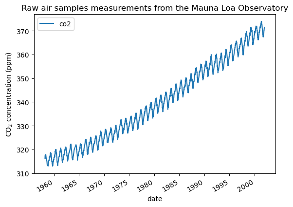
We will preprocess the dataset by taking a monthly average and drop month for which no measurements were collected. Such a processing will have an smoothing effect on the data.

# Resample data monthly
co2_data = co2_data.resample("M").mean().dropna(axis="index", how="any")

Cross validation is an important step in machine learning. In cross validation, the machine learning model is trained and evaluated on different subsets of input data. This step is crucial for clean evaluation, increased generalizability, and minimize underfitting & overfitting.

from sklearn.model_selection import train_test_split

RANDOM_SEED = 42  # Ensures reproducibility of split
co2_train, co2_validation = train_test_split(
    co2_data, test_size=0.25, shuffle=False, random_state=RANDOM_SEED
)

plt.plot(co2_train)
plt.plot(co2_validation)
plt.ylabel("Monthly average of CO$_2$ concentration (ppm)")
plt.xlabel("Date")
_ = plt.title(
    "Monthly average of air samples measurements\nfrom the Mauna Loa Observatory"
)
plt.legend(["train", "validation"])

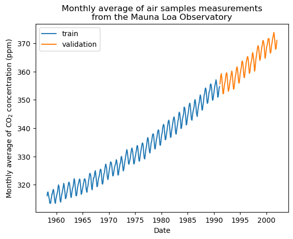
The idea in this example will be to predict the CO2 concentration in function of the date. We are as well interested in extrapolating for upcoming year after 2001.

As a first step, we will divide the data and the target to estimate. The data being a date, we will convert it into a numeric.

X = (co2_train.index.year + co2_train.index.month / 12).to_numpy().reshape(-1, 1)
y = co2_train["co2"].to_numpy()

Model fitting using Decision Tree Regression

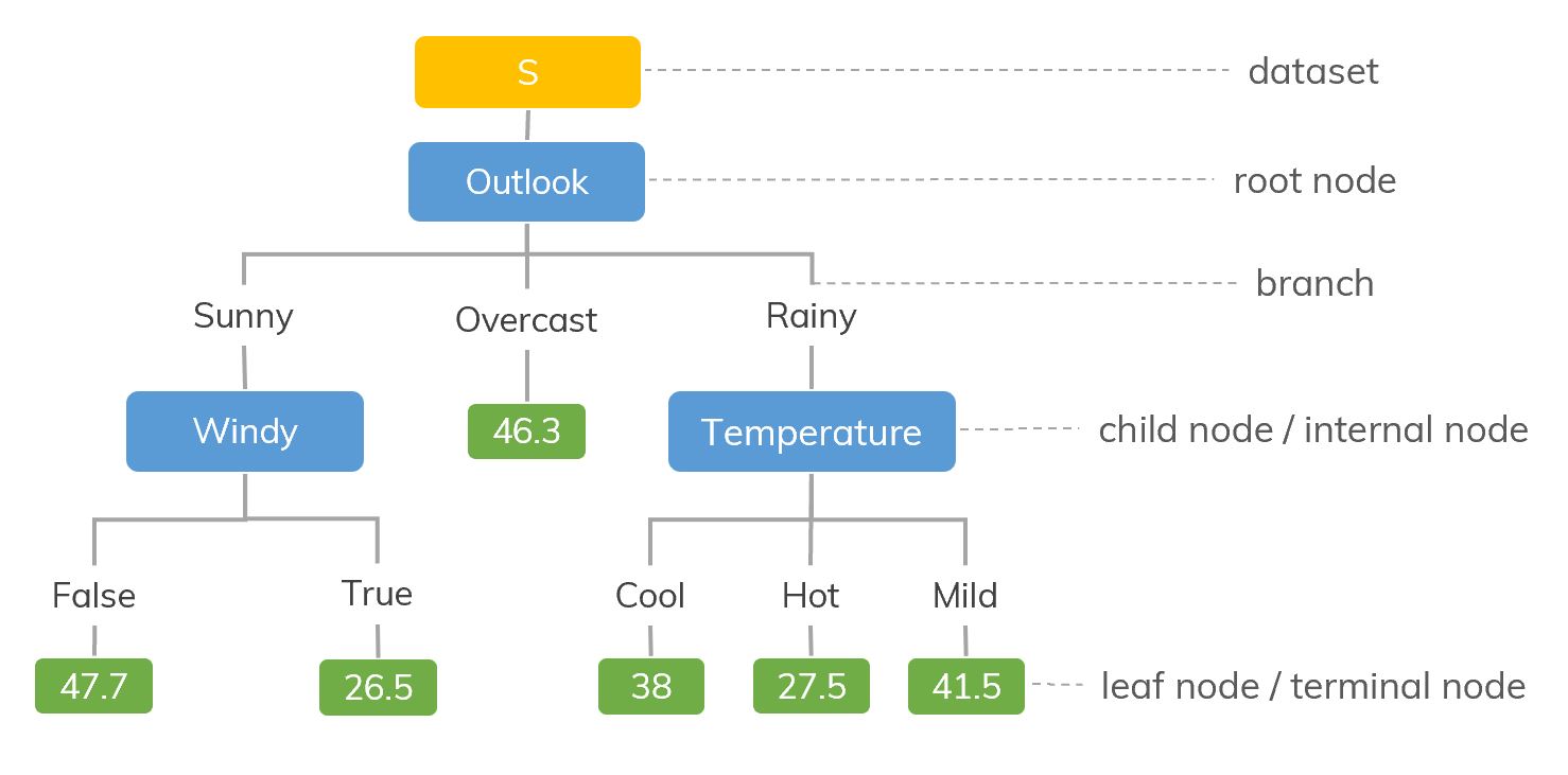
Decision Trees (DTs) are a non-parametric supervised learning method used for classification and regression. The goal is to create a model that predicts the value of a target variable by learning simple decision rules inferred from the data features. A tree can be seen as a piecewise constant approximation.

Decision trees learn from data to approximate a function with a set of if-then-else decision rules. The deeper the tree, the more complex the decision rules. Deeper trees are more powerful, but this can lead to overfitting.

from sklearn import tree

# Train models
decision_tree_1 = tree.DecisionTreeRegressor(max_depth=2)
decision_tree_2 = tree.DecisionTreeRegressor(max_depth=11)
decision_tree_1.fit(X, y)
decision_tree_2.fit(X, y)

Next, we evaluate the performance on the validation data.

# Make predictions on validation data
X_validation = (
    (co2_validation.index.year + co2_validation.index.month / 12)
    .to_numpy()
    .reshape(-1, 1)
)
y_validation = co2_validation["co2"].to_numpy()

y_predictions_1 = decision_tree_1.predict(X_validation)
y_predictions_2 = decision_tree_2.predict(X_validation)

from sklearn.metrics import mean_squared_error

# Calculate evaluation metrics
mse_of_regr_1 = mean_squared_error(y_validation, y_predictions_1)
mse_of_regr_2 = mean_squared_error(y_validation, y_predictions_2)

print(f"Validation MSE for Decision Tree with depth 2: {mse_of_regr_1:.4f}")
print(f"Validation MSE for Decision Tree with depth 11: {mse_of_regr_2:.4f}")

Out:
Validation MSE for Decision Tree with depth 2: 210.6841
Validation MSE for Decision Tree with depth 11: 96.5067

Now, we will use the the fitted models to predict on:

training data to inspect the goodness of fit;
validation data to inspect the generalizability;
future data to see the extrapolation done by the models.

Thus, we create synthetic data from 1958 to the current month.

import datetime
import numpy as np

# Get dates from 1958 to 2023
today = datetime.datetime.now()
current_month = today.year + today.month / 12
X_test = np.linspace(start=1958, stop=current_month, num=1_000).reshape(-1, 1)

# Make predictions
y_1 = decision_tree_1.predict(X_test)
y_2 = decision_tree_2.predict(X_test)

plt.figure(figsize=(10, 6))
plt.scatter(X, y, s=20, edgecolor="black", c="darkorange", label="data")

# Plot predictions of decision tree 1
plt.plot(X_test, y_1, color="cornflowerblue", label=f"max_depth={decision_tree_1.max_depth}", linewidth=2)

# Plot predictionso f decision tree 2
plt.plot(X_test, y_2, color="yellowgreen", label=f"max_depth={decision_tree_2.max_depth}", linewidth=2)

plt.xlabel("data")
plt.ylabel("target")
plt.title("Decision Tree Regression")
plt.legend()
plt.show()

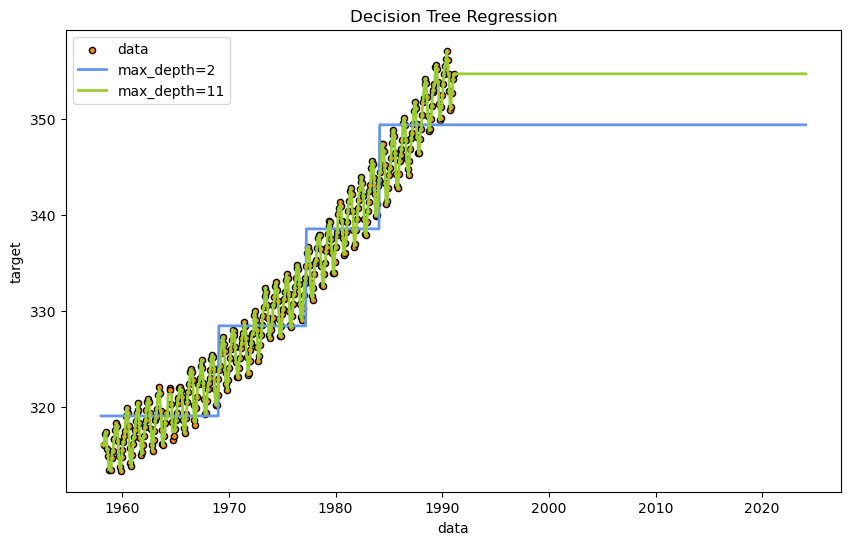
As you can see, the decision tree regression was able to fit data within the existing domain quite well. The criteria for decisions is intuitive and can be understood with a simple visualization. However, it has completely failed to predict any future trend outside the domain it was trained on.

Model the derivative of the data

To improve the model’s generalization, we will predict on differences in CO2 rather than absolute CO2 levels, using a “sliding window” of recent CO2 differences as the input. We will also normalize the data.

def preprocess_data(input_data, train_window, scaler, forecast_window=1, is_test=False):
    """
    Function that takes data and reformat for the autoregressive task
    """

    # Take derivative
    input_data = np.concatenate([[0], np.diff(input_data)])

    # Scale values
    scaler = scaler

    # Important: Not to leak information from training data to test data (clean evaluation)
    if is_test:
        normalized_data = scaler.transform(input_data.reshape(-1, 1)).reshape(-1)
    else:
        normalized_data = scaler.fit_transform(input_data.reshape(-1, 1)).reshape(-1)

    # Create input-output pairs
    in_seq = []
    out_seq = []
    L = len(normalized_data)

    # Reformat training data for autoregressive task
    for i in range(0, L - train_window - forecast_window, forecast_window):
        train_seq = normalized_data[i : i + train_window]
        train_label = normalized_data[
            i + train_window : i + train_window + forecast_window
        ]

        in_seq.append(train_seq)
        out_seq.append(train_label)

    return normalized_data, in_seq, out_seq, scaler

from sklearn.preprocessing import StandardScaler

# Paramters
TRAIN_WINDOW = 50  # No of months looked back
FORECAST_WINDOW = 1  # No of months predicted forward
standardScaler = StandardScaler()

# Create training data for autoregrssive task
normalized_train, X_train, y_train, scaler = preprocess_data(
    list(co2_train["co2"]),
    TRAIN_WINDOW,
    standardScaler,
    forecast_window=FORECAST_WINDOW,
    is_test=False,
)

We will train 3 decision trees at different max depths.

# Train models
decistion_tree_3 = tree.DecisionTreeRegressor(max_depth=2)
decistion_tree_3.fit(X_train, y_train)

decision_tree_4 = tree.DecisionTreeRegressor(max_depth=10)
decision_tree_4.fit(X_train, y_train)

decision_tree_5 = tree.DecisionTreeRegressor(max_depth=25)
decision_tree_5.fit(X_train, y_train)

Next, we will evaluate trained decision trees on the validation data.

# Create validation data for autoregrssive task
normalized_test, X_validation, y_validation, _ = preprocess_data(
    list(co2_validation["co2"]),
    TRAIN_WINDOW,
    standardScaler,
    forecast_window=FORECAST_WINDOW,
    is_test=True,
)

# Make predictions on validation data
y_predictions_3 = decistion_tree_3.predict(X_validation)
y_predictions_4 = decision_tree_4.predict(X_validation)
y_predictions_5 = decision_tree_5.predict(X_validation)

# Calculate evaluation metrics
mse_of_decision_tree_3 = mean_squared_error(y_validation, y_predictions_3)
mse_of_decision_tree_4 = mean_squared_error(y_validation, y_predictions_4)
mse_of_decision_tree_5 = mean_squared_error(y_validation, y_predictions_5)

print(f"Validation MSE for Decision Tree with depth 2: {mse_of_decision_tree_3:.4f}")
print(f"Validation MSE for Decision Tree with depth 10: {mse_of_decision_tree_4:.4f}")
print(f"Validation MSE for Decision Tree with depth 25: {mse_of_decision_tree_5:.4f}")

Out:
Validation MSE for Decision Tree with depth 2: 0.1530
Validation MSE for Decision Tree with depth 10: 0.1828
Validation MSE for Decision Tree with depth 25: 0.1621

Now we will generate test data that runs all the way to the present day to see the model’s predictions. We use the model’s own prediction as part of the sliding window for the next prediction, to extrapolate arbitrarily far into the future.

dates = pd.period_range("1958", "2023", freq="M").to_timestamp()

test_inputs = list(normalized_train)
future_predictions_3 = test_inputs.copy()
future_predictions_4 = test_inputs.copy()
future_predictions_5 = test_inputs.copy()

# Make predictions on validation data
future_predictions_count = len(dates) - len(test_inputs)

# Iteratively make predictions by moving the training window forward
for i in range(future_predictions_count):
    seq = future_predictions_3[-TRAIN_WINDOW:]
    prediction = decistion_tree_3.predict([seq])
    future_predictions_3.append(prediction[0])

    seq = future_predictions_4[-TRAIN_WINDOW:]
    prediction = decision_tree_4.predict([seq])
    future_predictions_4.append(prediction[0])

    seq = future_predictions_5[-TRAIN_WINDOW:]
    prediction = decision_tree_5.predict([seq])
    future_predictions_5.append(prediction[0])

Let’s plot the results. Note that it is still showing the differences (derivative) rather than the absolute value, and it’s still normalized.

plt.figure(figsize=(10, 6))

# Plots of derivative predictions
plt.plot(dates, future_predictions_3, label=f"max_depth={decistion_tree_3.max_depth}", linewidth=2)
plt.plot(dates, future_predictions_4, label=f"max_depth={decision_tree_4.max_depth}", linewidth=2)
plt.plot(dates, future_predictions_5, label=f"max_depth={decision_tree_5.max_depth}", linewidth=2)
plt.plot(dates[0:len(normalized_train)], normalized_train, label=f"true value", linewidth=2)

plt.xlabel("data")
plt.ylabel("target")
plt.title("Decision Tree Regression on Derivative")
plt.legend()
plt.show()

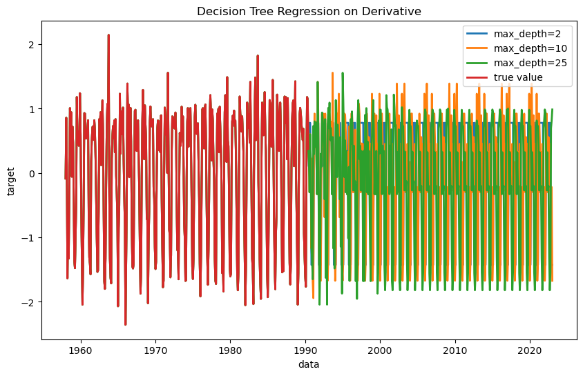
We can see that all of the decision trees are fitting the past data nearly perfectly, but do not entirely agree on future predictions.

Let’s convert the predictions back into absolute CO2 levels.

def postprocess_data(output_data, scaler, first_input):
    """
    Function to convert CO2 differences back to absolute CO2 levels
    """
    # Unscale the output
    output = scaler.inverse_transform(np.array(output_data).reshape(-1, 1)).reshape(-1)

    # Get cumulative sum
    output = np.cumsum(output) + first_input

    return output

# Post process data
decoded_3 = postprocess_data(future_predictions_3, scaler, list(co2_data["co2"])[0])
decoded_4 = postprocess_data(future_predictions_4, scaler, list(co2_data["co2"])[0])
decoded_5 = postprocess_data(future_predictions_5, scaler, list(co2_data["co2"])[0])

And plot the results:

plt.figure(figsize=(10, 6))

# Plot model outputs
plt.plot(dates, decoded_3, label=f"max_depth={decistion_tree_3.max_depth}", linewidth=2)
plt.plot(dates, decoded_4, label=f"max_depth={decision_tree_4.max_depth}", linewidth=2)
plt.plot(dates, decoded_5, label=f"max_depth={decision_tree_5.max_depth}", linewidth=2)

# Plot training and validation data
plt.plot(co2_train, label="train", linewidth=1)
plt.plot(co2_validation, label="validation", linewidth=1)

# Vertical dashed line to show the position of validation split
plt.axvline(co2_validation.index[0], linestyle="--", c="k")
plt.text(co2_validation.index[0], 320, "validation split", rotation=90)

# Vertical dashed line to show the position where future forecasts start
plt.axvline(co2_validation.index[-1], linestyle="--", c="k")
plt.text(co2_validation.index[-1], 320, "future forecasts start", rotation=90)

plt.xlabel("data")
plt.ylabel("target")
plt.title("Decision Tree Regression")
plt.legend()
plt.show()

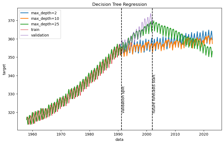
The results can vary quite a bit between runs. The method for fitting the decision trees is stochastic, and our many input variables are all similarly informative, so the tree’s hierarchy can vary significantly. Decision trees are not robust, so slight changes in input or in the tree structure can drastically alter predictions.

Recurrent Neural Networks - RNN

Long-Short Term Memory (LSTM) network

Training a Neural Network (NN) is computationally expensive. Training gets high resource consuming when the NN model is complex. Thus, we will use hardware acceleration (GPU) to speed up the computation.

# Check if GPU is available and set device
device = torch.device("cuda" if torch.cuda.is_available() else "cpu")
device

Out: device(type='cuda')

Hyperparameters are external configuration settings for a machine learning model that are not learned from the data but are set prior to training, influencing the model’s performance and behavior. Tuning hyperparameters for research projects require use of systematic approaches and packages (e.g. SHERPA, Optuna). However, we will do manual hyperparamter tuning (trial and error) for now.

# Define hyperparameters
TRAIN_WINDOW = 84
FORECAST_WINDOW = 1

input_size = TRAIN_WINDOW  # Input layer size
hidden_size = 32  # No of hidden layer neurons
output_size = FORECAST_WINDOW  # Output layer size

n_hidden_layers = 1
num_epochs = 75  # Number of training epochs
learning_rate = 0.005

Then, we will reformat the input data for the autoregressive task using LSTM.

standardScaler = StandardScaler()

# Generate training data for RNN
normalized_train, X_train, y_train, scaler = preprocess_data(
    list(co2_train["co2"]),
    TRAIN_WINDOW,
    standardScaler,
    forecast_window=FORECAST_WINDOW,
    is_test=False,
)

# Generate validation data for RNN
normalized_validation, X_validation, y_validation, scaler = preprocess_data(
    list(co2_validation["co2"]),
    TRAIN_WINDOW,
    standardScaler,
    forecast_window=FORECAST_WINDOW,
    is_test=True,
)

There are different python frameworks for building neural network models. Two most popular ones are:

PyTorch
TensorFlow

We will use PyTorch in this example. First, we need to convert data to be feasible with PyTorch.

# PyTorch
import torch
import torch.nn as nn
import torch.optim as optim
from torch.utils.data import DataLoader, TensorDataset

# Convert data to tensors and transfer to GPU (if available)
X_train_tensor = torch.Tensor(np.array(X_train)).to(device)
y_train_tensor = torch.Tensor(np.array(y_train)).to(device)

X_validation_tensor = torch.Tensor(np.array(X_validation)).to(device)
y_validation_tensor = torch.Tensor(np.array(y_validation)).to(device)

After that, we define the LSTM model and instantiate other model configuration parameters. Out of these optimizer and loss function are two important configurations that affect the trained LSTM model.

# Define the LSTM model
class SimpleLSTM(nn.Module):
    def __init__(self, input_size, hidden_size, output_size):
        super(SimpleLSTM, self).__init__()
        # Define LSTM model
        self.lstm = nn.LSTM(input_size, hidden_size, num_layers=n_hidden_layers).to(
            device
        )
        self.fc = nn.Linear(hidden_size, output_size)

    def forward(self, x):
        out, _ = self.lstm(x)
        out = self.fc(out)
        return out

# Instantiate the model, loss function, and optimizer
model = SimpleLSTM(input_size, hidden_size, output_size).to(device)
loss_function = nn.MSELoss()
optimizer = optim.Adam(model.parameters(), lr=learning_rate)

Afterward, we train the LSTM model for multiple epochs (epoch = single pass through the entire training dataset during the training).

# Training loop
for epoch in range(num_epochs):
    # Forward pass
    output = model(X_train_tensor)

    # Compute the loss
    loss = loss_function(output, y_train_tensor)

    # Backward pass and optimization
    optimizer.zero_grad()
    loss.backward()
    optimizer.step()

    # Print the loss every 25 epochs
    if (epoch + 1) % 25 == 0:
        print(f"Epoch [{epoch + 1}/{num_epochs}], Loss: {loss.item():.4f}")

Then, we make evaluate the trained model on validation data.

# Make predictions on validation data
with torch.no_grad():
    y_predictions_rnn = model(X_validation_tensor)

# Calculate evaluation metrics
mse_of_rnn = mean_squared_error(y_validation_tensor.cpu(), y_predictions_rnn.cpu())

print(f"Validation MSE for RNN: {mse_of_rnn:.4f}")

Out: Validation MSE for RNN: 0.0710

Next, we make predictions on train data, validation data and extrapolate to future data similar to the way we did in decision trees example.

dates = pd.period_range("1958", "2023", freq="M").to_timestamp()
test_inputs = list(normalized_train)

# Number of predictions to make
future_predictions_count = int(
    np.ceil((len(dates) - len(test_inputs)) / FORECAST_WINDOW)
)

# Iteratively make predictions by moving the training window forward
for i in range(future_predictions_count):
    # Get the last set of input features
    X_test = torch.Tensor(X_train[-1]).view(1, -1).to(device)
    # Get the last target variable
    y_test = torch.Tensor(y_train[-1]).to(device)

    # Predict forecast window forward
    with torch.no_grad():
        y_pred = model(X_test)

    # Append current y values to X
    X_train.append(
        torch.cat((X_test[0][-(TRAIN_WINDOW - FORECAST_WINDOW) :], y_test))
        .cpu()
        .data.numpy()
    )

    # Append prediction to the target values
    y_train.append(y_pred.cpu().data.numpy()[0])

# First value (0) + first values in first training data
#       + y values in y_train (e.g. forecast window values)
predictions = (
    [np.array(0)]
    + [np.array(value) for value in X_train[0]]
    + [np.array(value) for y in y_train for value in y]
)

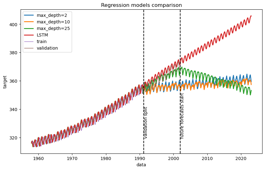
Finally, we convert CO2 derivates to absolute CO2 levels and compare with the results we got with Decision Trees.

# Post process data
decoded = postprocess_data(predictions, scaler, list(co2_train["co2"])[0])

dates = pd.period_range("1958", "2023", freq="M").to_timestamp()
plt.figure(figsize=(10, 6))

# Plots for model predictions
plt.plot(dates, decoded_3, label=f"max_depth={decistion_tree_3.max_depth}", linewidth=2)
plt.plot(dates, decoded_4, label=f"max_depth={decision_tree_4.max_depth}", linewidth=2)
plt.plot(dates, decoded_5, label=f"max_depth={decision_tree_5.max_depth}", linewidth=2)
plt.plot(dates, decoded[: len(dates)], label=f"LSTM", linewidth=2)

# Plot training and validation data
plt.plot(co2_train, label="train", linewidth=1)
plt.plot(co2_validation, label="validation", linewidth=1)

# Vertical dashed line to show the position of validation split
plt.axvline(co2_validation.index[0], linestyle="--", c="k")
plt.text(co2_validation.index[0], 320, "validation split", rotation=90)

# Vertical dashed line to show the position where future forecasts start
plt.axvline(co2_validation.index[-1], linestyle="--", c="k")
plt.text(co2_validation.index[-1], 320, "future forecasts start", rotation=90)

plt.xlabel("data")
plt.ylabel("target")
plt.title("Regression models comparison")
plt.legend()
plt.show()

# Print evaluation metrics for comparison
print(f"Validation MSE for Decision Tree with depth 2  : {mse_of_decision_tree_3:.4f}")
print(f"Validation MSE for Decision Tree with depth 10 : {mse_of_decision_tree_4:.4f}")
print(f"Validation MSE for Decision Tree with depth 25 : {mse_of_decision_tree_5:.4f}")
print(f"Validation MSE for Recurrent Neural Network    : {mse_of_rnn:.4f}")

Based on the visualization and validation mean squared error, it is clear that LSTM (RNN) model successfully fits the training data, and extrapolate to future learning the underlying pattern unlike decision tree models.

For more information

Attribution:

This workshop was modified from the following:

Gaussian process regression (GPR) on Mauna Loa CO2 data

Rasmussen, Carl Edward. “Gaussian processes in machine learning.” Summer school on machine learning. Springer, Berlin, Heidelberg, 2003.

Authors:

Jan Hendrik Metzen jhm@informatik.uni-bremen.de
Guillaume Lemaitre g.lemaitre58@gmail.com

License: BSD 3 clause

Resources and Further Reading

Bio Break! We will start again at 3:00 PM.