7. Real Example Cleanup
![]()
Overview
Questions
- How do you clean an example dataset?
- How do you deal with missing data?
- How do you fix column type mismatches?
Objectives
- Clean an example dataset using both previously described concepts and some new ones.
Cleaning Real Data
The previous episodes have focused on key concepts with small datasets and/or made-up data. However, these examples can only take you so far. For this reason, the remaining lessons and examples will be focused on an actual dataset from the Hawaiian Ocean Time-Series (HOT) data website (Link to HOT Data Website). This website allows you to query data generated by the time series through various modules.
The Hawaiian Ocean Time Series has been collecting samples from station ALOHA located just North of Oahu since 1988. The map below shows the exact location where the samples we will be using originate from.

(Original image from: https://www.soest.hawaii.edu/HOT_WOCE/bath_HOT_Hawaii.html)
Going forward we are going to be using data from HOT between the 1st of January 2010 to the 1st of January 2020. This particular data we are going to be utilizing comes from bottle extractions between depths from 0 to 500m. The environmental variables that we will be looking at include:
| Column name | Environmental Variable |
|---|---|
| botid # | Bottle ID |
| date mmddyy | Date |
| press dbar | Pressure |
| temp ITS-90 | Temperature |
| csal PSS-78 | Salinity |
| coxy umol/kg | Oxygen concentration |
| ph | pH |
| phos umol/kg | Phosphate concentration |
| nit umol/kg | Nitrate + Nitrite concentration |
| no2 nmol/kg | Nitrite concentration |
| doc umol/kg | Dissolved Organic Carbon concentration |
| hbact # 1e5/ml | Heterotrophic Bacteria concentration |
| pbact # 1e5/ml | Prochlorococcus numbers |
| sbact # 1e5/ml | Synechococcus numbers |
The data contains over 20000 individual samples. To analyze the data we are going to clean it up. Then, in the next episode we will analyze and visualize it. To do this, we will be using some of the tricks we have already learned while also introducing some new concepts. Note: The dataset we are using has been modified from its original format to reduce the amount of cleaning up we need to do.
Cleaning Up
DataFrame Content Cleanup
During our initial clean up we will only load in the first few rows of our datasets entire DataFrame. This will make it easier to work with and less daunting.
pd.read_csv("./data/hot_dogs_data.csv", nrows=5)
This will show us the DataFrame seen below:
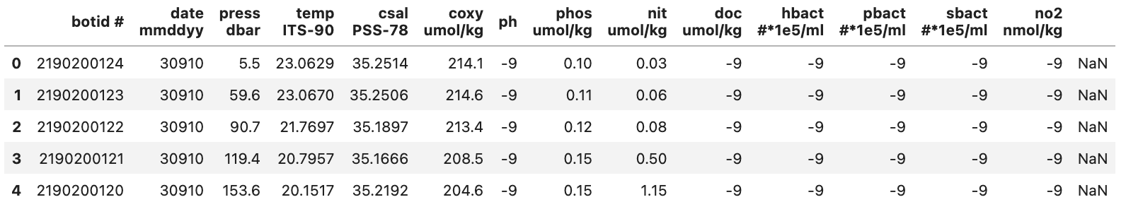
From this we can see a few things:
- There are a lot of -9 values
- This is likely to denote Null values in the dataset
- The last column (to the right of the no2 column) doesn’t seem to contain a header or any data
Both of these issues can easily be fixed using Pandas and things we’ve learned previously.
To start off let’s fix the first problem we saw which was the large number of -9 values in the dataset. These are especially strange for some of the columns e.g. how can there be a negative concentration of hbact i.e. heterotrophic bacteria? This is a stand-in for places where no measurement was obtained.
Exercise: Treating -9 values as NaN values when loading data
To start off try fixing the read_csv() method so that all -9 values are treated as NaN values.
Solution
To fix this we can add the parameterna_values= -9 to the read_csv() method giving us the following code bit:
pd.read_csv("./data/hot_dogs_data.csv", nrows=5, na_values=-9)
Below shows how our DataFrame now looks:
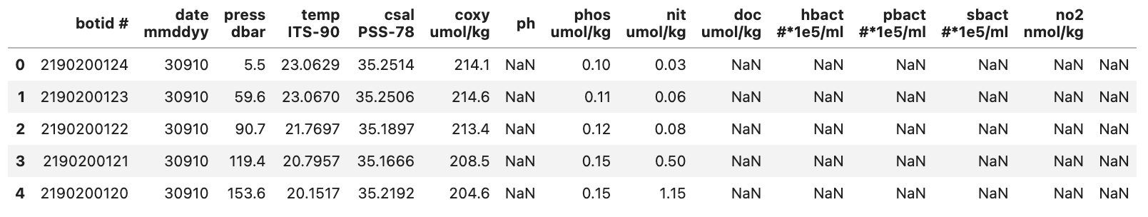
With this, we have fixed the problematic -9 values from our initial DataFrame.
Temperature Column
The temperature column could technically contain -9 values. However, all temperature measurements were above 0 so this is not an issue.
The second problem we identified was that there was an extra column (with no header) made up of only NaN values. This is probably an issue with the original file and if we were to take a look at the raw .csv file we find that each row ends with a ‘,’. This causes read_csv to assume that there is another column with no data since it looks for a new line character (\n) to denote when to start a new row.
There are various methods to deal with this. However, we are going to use a relatively simple method that we’ve already learned. As we discussed in a previous episode pandas DataFrames has a method to drop columns (or indexes) called drop. When provided with the correct arguments, it can drop a column based on its name. Knowing this we can chain our read_csv method with the drop method so that we load in the blank column and then immediately remove it.
Exercise: Dropping the blank column
The final command we will be using can be seen below. However, the columns parameter is missing any entries in its list of columns to drop. You will be fixing this by adding the name of the column that is empty (hint: the name isn’t empty).
pd.read_csv("./data/hot_dogs_data.csv", nrows=5, na_values=-9).drop(columns=[])
To get the name of the column we will want to utilize a DataFrame attribute that we have already discussed that provides us with the list of names in the same order they occur in the DataFrame.
Solution
To get the name of the columns we can simply access thecolumns, Series attribute that ever DataFrame has. This can be done either through chaining it after our read_csv method or by store it in a variable and then call the method using that variable. Below we use the chain approach.
pd.read_csv("./data/hot_dogs_data.csv", nrows=5, na_values=-9).columns
  Index(['botid #', ' date mmddyy', ' press dbar', ' temp ITS-90',
   ' csal PSS-78', ' coxy umol/kg', ' ph', ' phos umol/kg', ' nit umol/kg',
   ' doc umol/kg', ' hbact #*1e5/ml', ' pbact #*1e5/ml', ' sbact #*1e5/ml',
   ' no2 nmol/kg', ' '],
  dtype='object')
The last entry in the
Series is our 'blank' column i.e. `' '`. We add this as the only entry to our drop method and get the following code bit.
pd.read_csv("./data/hot_dogs_data.csv", nrows=5, na_values=-9).drop(columns=[" "], axis=1)
This then gives us the output DataFrame seen below:
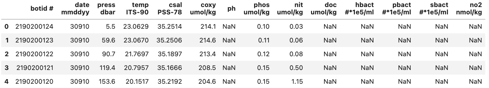
We now have fixed some of the initial issues related to our dataset. It should be noted that there might still exist other issues with our dataset since we have only relied on the first few rows.
Column Names
Checking the columns attribute even if nothing immediately looks wrong can be good in order to spot e.g. blank spaces around column names that can lead to issues.
One final thing that we are going to do that is not quite “clean up” but nonetheless important is to set our index column when we load the data. The column we are going to use for this is the ‘botid #’ column. We can also remove the nrows=5 parameter since we want to load the whole DataFrame starting in the next section.
Exercise: Setting the index column when loading data
To set the index column we can use a parameter in read_csv that was mentioned in a previous episode. See if you can remember it!
Solution
To set the index column when we load the data we just have to add the parameterindex_col and set it to botid #. Note: we have removed the nrows=5 parameter in the code bit below since we no longer need it.
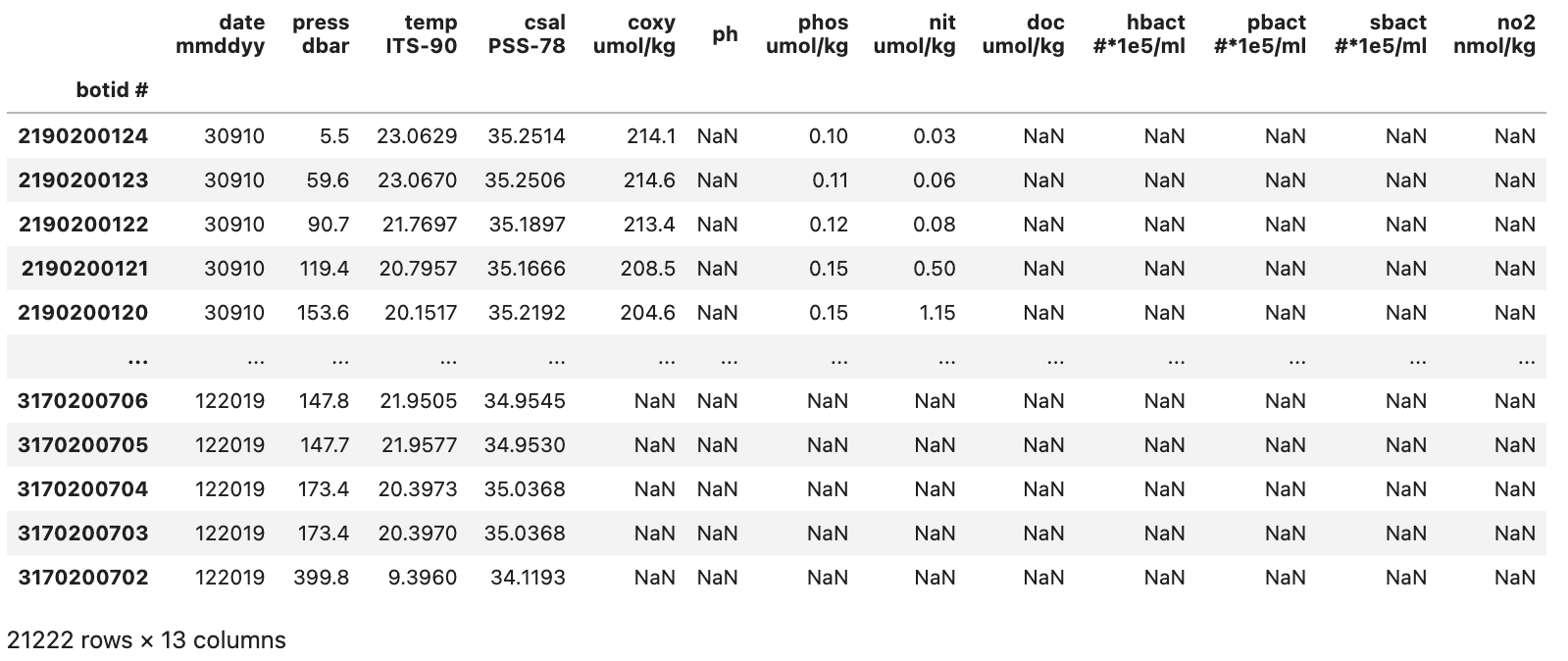
pd.read_csv("./data/hot_dogs_data.csv", na_values=-9, index_col="botid #").drop(columns=[" "], axis=1)
This gives us a somewhat cleaned up DataFrame that looks like the image below:
With our initial cleanup done we can now save the current version of our DataFrame to the df variable. This df variable will be used for the next two sections.
DataFrame Column Types
Now that we have fixed the initial issues we could glean from an initial look at the data we can take a look at the types that Pandas assumed for each of our columns. To do this we can access the .dtypes attribute.
Python
df.dtypes
Output
 date mmddyy         int64
 time hhmmss         int64
 press dbar        float64
 temp ITS-90       float64
 csal PSS-78       float64
 coxy umol/kg      float64
 ph                float64
 phos umol/kg      float64
 nit umol/kg       float64
 doc umol/kg       float64
 hbact #*1e5/ml    float64
 pbact #*1e5/ml    float64
 sbact #*1e5/ml    float64
 no2 nmol/kg       float64
dtype: object
Most of the columns have the correct type with the exception of the ‘date mmddyy’ column that has the int64 type. Pandas has a built in type to format date and time columns and conversion of the date column to this datetime type will help us later on.
To change the type of a column from an int64 to a datetime type is a bit more difficult than e.g. a int64 to float64 conversion. This is because we both need to tell Pandas the type that we want it to convert the column’s data to and the format that it is in. For our data, this is MMDDYY which we can give to Pandas using format='%m%d%y'. This format parameter can be very complicated but is based on native Python more information can be found on the to_datetime method docs (Link to datetime method docs).
The code bit below creates a new column called ‘date’ that contains the same data for each row as is found in the ‘date mmddyy’ column but instead with the datetime64 type. It will not delete the original ‘date mmddyy’ column.
Python
df["collection_date"] = pd.to_datetime(df['date mmddyy'], format='%m%d%y')
df.dtypes
Output
date mmddyy                int64
time hhmmss                int64
press dbar               float64
temp ITS-90              float64
csal PSS-78              float64
coxy umol/kg             float64
ph                       float64
phos umol/kg             float64
nit umol/kg              float64
doc umol/kg              float64
hbact #*1e5/ml           float64
pbact #*1e5/ml           float64
sbact #*1e5/ml           float64
no2 nmol/kg              float64
date              datetime64[ns]
dtype: object
We can see from the output that we have all of our previous columns with the addition of a ‘date’ column with the type datetime64. If we take a look at the new column we can see that it has a different formatting compared to the ‘date mmddyy’ column
Python
df["collection_date"]
Output
botid #
2190200124   2010-03-09
2190200123   2010-03-09
2190200122   2010-03-09
2190200121   2010-03-09
2190200120   2010-03-09
                ...
3170200706   2019-12-20
3170200705   2019-12-20
3170200704   2019-12-20
3170200703   2019-12-20
3170200702   2019-12-20
Name: collection_date, Length: 21222, dtype: datetime64[ns]
Now that we’ve added this column (which contains the same data as found in ‘date mmddyy’ just in a different format) there is no need for the original date mmddyy column so we can drop it.
Python
df = df.drop(columns=["date mmddyy"])
DataFrame Overview
A final thing we will want to do before moving on to the analysis episode is to get an overview of our DataFrame as a final way of checking to see if anything is wrong. To do this we can use the describe() method which we discussed earlier.
Python
df.describe()
Output
         time hhmmss    press dbar   temp ITS-90   csal PSS-78  coxy umol/kg  \
count   21222.000000  21222.000000  21222.000000  21210.000000   3727.000000
mean   103238.977523    119.381105     21.570407     35.020524    198.222297
std     68253.013809    120.193833      4.961006      0.382516     27.787824
min         3.000000      0.800000      6.055800     34.018800     30.900000
25%     40625.000000     25.500000     20.625800     34.922500    199.350000
50%    101309.000000     89.700000     23.109450     35.138700    207.200000
75%    154822.000000    150.900000     24.742175     35.281500    212.000000
max    235954.000000    500.000000     28.240100     35.556400    230.900000

               ph  phos umol/kg  nit umol/kg  doc umol/kg  hbact #*1e5/ml  \
count  885.000000   2259.000000  2253.000000   868.000000      750.000000
mean     7.956939      0.448331     5.505113    63.688341        3.933479
std      0.158210      0.638772     9.159562    10.287748        1.173908
min      7.366000      0.000000     0.000000    41.270000        1.481000
25%      7.898000      0.070000     0.020000    55.467500        2.976250
50%      8.035000      0.120000     0.240000    67.395000        4.042000
75%      8.065000      0.520000     6.620000    72.282500        4.809500
max      8.105000      2.610000    35.490000    80.460000        7.889000

       pbact #*1e5/ml  sbact #*1e5/ml  no2 nmol/kg
count      749.000000      750.000000          0.0
mean         1.364606        0.010932          NaN
std          0.938620        0.011851          NaN
min          0.000000        0.000000          NaN
25%          0.337000        0.000000          NaN
50%          1.643000        0.009000          NaN
75%          2.176000        0.016000          NaN
max          3.555000        0.091000          NaN
A look at the output shows us that the ‘no2 nmol/kg’ column does not contain any useable data based on its count value being 0. Since this column doesn’t contain any information of interest we can drop it to clean up our DataFrame.
Python
df = df.drop(columns=["no2 nmol/kg"])
With this done, our data is reasonably cleaned up and we have the DataFrame seen in the image below:
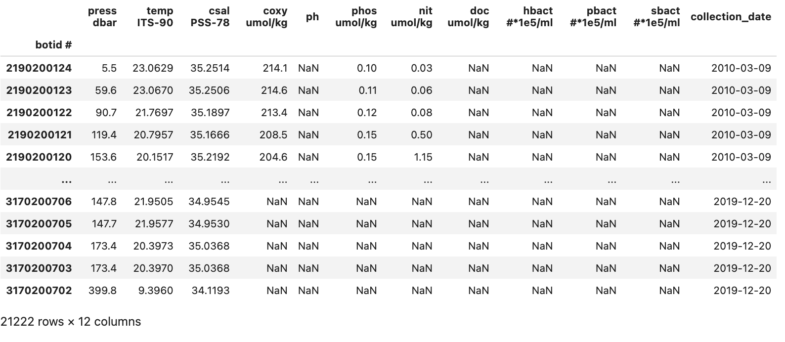
We can now move on to the analysis and visualization of the data in our DataFrame.
Summary
With this we’ve cleaned up our initial dataset. To summarize we have:
- Replaced the -9 placeholder for Null values with NaN values
- Fixed an issue with an extra column containing no data
- Added a custom row index
- Converted the data in ‘date mmddyy’ to a Pandas-supported datetime type
- Dropped two columns:
- ‘date mmddyy’ column since the new ‘date’ column contains the same data but in a better type
- ‘no2 nmol/kg’ column since it contained no data
Key Points
- Cleaning a dataset is an iterative process that can require multiple passes.
- Restart the kernel when cleaning a dataset to make sure that your code encompasses all the cleaning needed.