3. Loading and Handling Pandas Data

Pandas Data Structures

You can follow along using the Jupyter Notebook associated with this module linked to from the Open in Colab button above.

Before we start loading data into Pandas we need to become familiar with two primary data structures used in Pandas:

• Series
• DataFrames

One of the primary benefits of Series and DataFrames over native python data structures is that it is a very natural way to describe a data set by referencing the rows and columns of the data.

Pandas Series Vs. DataFrames

Pandas has two principal data structures, Series and DataFrames. If you are familiar with Microsoft’s Excel, then you can consider Series to a single column in an Excel sheet and DataFrames to entire tables (or spreadsheets).

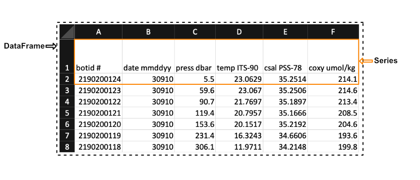
We see in the image above that a Series in the context of Excel could be the first row of the spreadsheet, while a DataFrames would be the entire spreadsheet. In other words, a DataFrames is simply a collection of labeled Series.

Pandas Data Types

When creating a Series Pandas will store all the data as the same type. The mapping from the native Python types to what they would be in Pandas is summarized below.

Pandas DataFrames Basics

Reiterating the example mentioned earlier, it helps to think of DataFrames as MS. Excel spreadsheets where each row (or column) is an individual Series. Just like Excel spreadsheets, which typically have row and column labels (numbers for the rows and letter for the columns), DataFrames also have two associated Index objects, one to label rows and another to label columns.

DataFrames may be generated either by importing a data file, such as a CSV, or by transitioning a current Python data structure into a dataframe. Here, we will focus on creating a DataFrame by ingesting data from a file.

Import the Pandas Package

Pandas is traditionally imported with the shortcut, or alias, pd.

import pandas as pd

Loading and Parsing Data

Pandas can be used to load data from a variety of file formats. The most common ones fall into one of the following two categories: Delimited and Fixed Width

• Delimited files are organized such that columns and rows are separated by a certain character called a delimiter
• Fixed-width files are those where each entry in a column has a fixed number of characters

We will focus on the delimited .csv file type. The CSV acronym stands for ‘Comma Separated Values’ and informs us that the column entries are delimited by commas and the rows are delimited by a new line. So, the example we discussed in this cell conforms to the .csv format.

Pandas provides a suite of functions to parse input data into DataFrames. The function read_csv() can read any character-delimited text file into DataFrames. To use read_csv(), we need to at least provide the path of the input file. For example, if we aim to read a file named my_input_file.csv in the notebook’s current directory and assign the data to a new DataFrame, df, the command would be: df = pd.read_csv(my_input_file.csv).

Pandas provides various optional parameters that may be set when calling the read_csv() function. To learn more, see the read_csv() documentation, which summarizes all of the parameters. We will be covering many of the most important parameters throughout the rest of this module.

By default read_csv() will separate data entries when it encounters a comma and will separate rows by new lines encoded by ‘\n’. If we wanted to change this behavior so that read_csv() separates by tabs (encoded with \t), then we can set the optional parameter sep = '\t'. Therefore, to read the data in the file ‘tsv_example.tsv’, which is a tab separated values file, and save the data in a Pandas DataFrame called df, then we would type:

df = pd.read_csv('data/tsv_example.tsv', sep='\t')

Though read_csv() can handle .tsv files, there is a specific parsing function for .tsv files: read_table(). The read_table() documentation is available at this link.

In the previous examples, we loaded into a Pandas DataFrame the entire dataset. However, when working with large datasets it is good practice to initially load and explore a small chunk before loading the entire dataset to ensure that the file is parsed correctly. Small data sets are more manageable and errors are easier to spot, while large data sets take more time to parse. So, a good workflow is to read a small portion of the data and analyze the resulting data frame to see if you need to modify any of the default behaviors of the read function.

To load only up to a limited number of rows we can use the nrows parameter for both read_table() and read_csv(). For example, the sample file E3_tara_w1.csv is a csv file with a little over 200 rows, but if we wanted to read only the first 5 rows of this file we can call the Pandas read_csv() function and set nrows = 5. We can then use the DataFrame attribute (property or characteristic accessible using the dot notation).

df = pd.read_csv('data/tsv_example.tsv', nrows=5)
df.shape # Returns the number of rows and columns of the DataFrame 'df' (rows, columns)

(5, 7)

We see that the DataFrame df, that we saved the data in, has a shape attribute of (5, 7). This means that there are 5 rows (since we set nrows=5) and 7 columns (all the columns of the dataset).

Headers and Indexes

df = pd.read_csv("data/noheader_example.csv", header=None)
df

However, this does not mean that the DataFrame does not have headers but rather that Pandas will set them to be an integer value. An example is shown in the figure below:

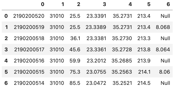
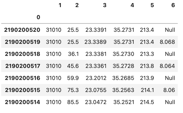
You might also notice that there is also a corresponding integer number in the far left side of each row. This is the index that is essentially the “index” representing each row. If we have a column that is specific to each row in the Python file we can tell Pandas to use that column instead of the default of using an integer. This can be done by e.g. setting index_col='unique_id' however, if you don’t have any headers you can also specify the column by using its integer location e.g. index_col=0. Note that the integer location of a column goes from left to right and starts at 0.

df = pd.read_csv('data/noheader_example.csv', header=None, index_col=0)
df

Common Data Loading Problems

Though data storage in plain text files should follow certain formats like .csv for ‘Comma Separated Values’ and .tsv for ‘Tab Separated Values’, there is still some ambiguity on how things like missing entries, and comments should be denoted. Below we will go through two examples of common issues when loading in data.

Missing Values

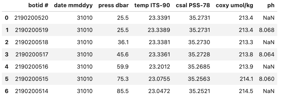
real-world data often contain missing values. These missing entries may be identifiable in the dataset by a number of different tags, like ‘NA’, ‘N.A.’, ‘na’, ‘missing’, etc. It is important to properly identify missing values when creating a DataFrame since certain DataFrame methods rely on the missing values being accounted for. For example, the count() method of a DataFrame returns the number of non-missing values in each column. If we want this to be an accurate count, then we need to be sure of pointing out all the tags, which represent ‘missing’ to Pandas.

As an example, to inform Pandas that missing values in a dataset are represented by the “Null” string value, you can specify na_values=’Null’ while reading the data file. In response, Pandas will substitute these missing values with NaN, which stands for “Not a Number” and carries significance in Python syntax.

df = pd.read_csv("data/null_values_example.csv", na_values='Null')
df

Without na_values='Null':

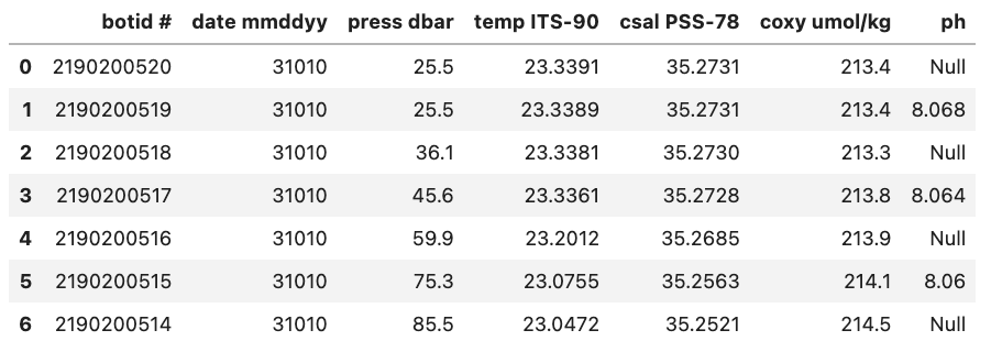
With na_values='Null':

Auto NaN values

Pandas will interpret certain values as being NaN values even without user Python. For example if ‘NULL’ is found then Pandas will treat it as a missing value and treat it as a NaN value.

Writing Data in Text Format

When using Pandas’ read_<filetype>() to import files into DataFrames, the complementary operation for exporting DataFrames to files uses the to_<filetype>() methods. Here, we will use to_csv(), which has a sole required parameter the output file name. This function will either create a new file or overwrite an existing one. The method to_csv() has several optional parameters for customization, all of which are detailed in the Pandas documentation for your reference.

df.to_csv('data/new_file.csv')

Key Points

Exercise: Loading An Excel File

---

Try it yourself! Load the first 10 lines of the Excel file ‘20_sales_records.xlsx’ into a variable and then display your DataFrame using the .head() method. Can you identify the number of rows and columns in the DataFrame.

• The file can be opened directly from the following URL: https://github.com/mahdi-b/change-hi.github.io/raw/main/morea/data-wrangling-1/Notebook/data/20_sales_records.xlsx.
• Click on the folder to the left side.
• After downloading the file (20_sales_records.xlsx), drag and drop it in the Files section to the left side of your Colab Notebook.
• Use the appropriate read_<file_> method along with the argument you learned to only parse 10 rows.
• This file has NaN values that are not automatically detected. They are labeled as 'none'. Have Pandas interpret these as NaN values upon loading of the dataset.
• Display the results.
• Identify the number of rows and columns of your resulting DataFrame.

Solution

'20_sales_records.xlsx' is an excel file containing 20 rows of data, but we only want Pandas to parse the first 10 rows. In addition, we want to interpret exisitng 'none' values as `NaN` values. This can all be accomplished with the following line of code:

    sales_df = pd.read_excel('data/20_sales_records.xlsx', nrows=10, na_values='none')  
  

The DataFrame should look like the following:

Use the method `.shape` to verify that `DataFrame` should have 10 rows, 14 columns, and `NaN` values replacing the 'none' values.

    sales_df.shape