4. Accessing and Subsetting Data
![]()
Overview
Questions
- How can you select individual columns or rows from a
DataFrame? - How can you subset a
DataFrame? - How can you sort a
DataFrame?
Objectives
- Learn how to select specific columns or rows from a
DataFrame - Learn how to select rows based on conditions.
- Learn how to sort a
DataFrame’s rows or columns.
Selection, Subsetting and Sorting a DataFrame
When exploring our data we will often want to modify specific rows, columns, or entries that satisfy certain conditions. We may want to either look at a single column of the data or work with a subset of the original data. Furthermore, it is often helpful to sort our data set using a particular relation to identify patterns and to understand the data’s structure. For example, suppose the original dataset we acquire and want to analyze describes a sports team’s performance for each game during a season and its original order is chronological. It may be interesting to sort the gameplay statistics using a different relation such as number of points scored to easily identify high and low-scoring games.
As with previous modules, you should follow along in the notebook, which can be opened by clicking the Open in Colab button above.
Selection
Selecting data from a DataFrame is intuitive and builds on concepts we discussed in the previous module. A DataFrame holds column names, called headers, and row names, called indexes. Depending on how we loaded the data these might be integers, strings (text) or combinations of both.
In the context of the table shown in the image below, Pandas allows us to choose specific combinations of rows and columns from the associated DataFrame. We will cover some ways to do that in the sections that follow:
Selecting Columns
To begin, let’s concentrate on subsetting columns. This operation closely resembles accessing keys in a Python dictionary. Thus, if we possess a DataFrame named df with a column labeled 'ph', we can subset the DataFrame by employing df['ph'].
Python
df['ph']
Output
Sample ID
Sample-1    7.951
Sample-2      NaN
Sample-3      NaN
Sample-4    7.780
Sample-5      NaN
Sample-6      NaN
Sample-7      NaN
Sample-8    7.496
Name: ph, dtype: float64
Selecting Rows
If on the other hand, we want to access a subset rows we have to use a slightly different approach. Previously, we could just pass the name of the column inside brackets if we want to access one or more rows we need to use the .loc or .iloc methods.
The first abbreviation, ‘loc,’ represents ‘location’ and requires you to specify the names of the rows you wish to access. The second abbreviation, ‘iloc,’ represents ‘integer location’ and requires you to provide the row index (a numerical value). Both methods can be set to retrieve the complete row(s), or only a subset of values associated with columns of interest.
So if we again have a DataFrame called df and a row called ‘Sample-1’ we can access it using df.loc['Sample-1', df.columns].
Python
df.loc['Sample-1', df.columns]
Output
date mmddyy     40610.0000
press dbar        239.8000
temp ITS-90        18.9625
csal PSS-78        35.0636
coxy umol/kg           NaN
ph                  7.9510
Name: Sample-1, dtype: float64
The attribute columns in the expression df.columns is used to retrieve all the header names (column labels) within the DataFrame referred to as df. It is employed above to inform Pandas that the column values within the DataFrame corresponding to the row labeled ‘Sample-1’ should be accessed.
If we were to use .iloc instead of .loc for the previous example and we know that ‘Sample-1’ is at index position 0 we would use df.iloc[0, :] and get the same result. You might notice that we also had to change df.columns to : when we used .iloc this is because df.columns provides the names of all the headers which is fine to do with .loc but not .iloc since the latter requires indexes, not names (strings).
Python
df.iloc[0, :]
Output
date mmddyy     40610.0000
press dbar        239.8000
temp ITS-90        18.9625
csal PSS-78        35.0636
coxy umol/kg           NaN
ph                  7.9510
Name: Sample-1, dtype: float64
The : operator: refresher
When used inside brackets, the : operator will return the range between the two values it is given. For example, if we had a Python list x with the following values [‘a’, ‘b’, ‘c’, ‘d’, ‘e’] and wanted to select ‘b’, ‘c’, and ‘d’ we can do this very concisely using the : operator.
Python
x = ['a', 'b', 'c', 'd', 'e']
x[2:5]
With the output:
['c', 'd', 'e']
Selecting Columns and Rows Simultaneously
As we saw in the previous section we can select one or more rows and/or columns to view. For example, if we wanted to view the ‘ph’ entry of ‘Sample-1’ from the previous example we could use .loc in the following manner.
Python
df.loc['Sample-1', 'ph']
Output
7.951
If we wanted to select multiple columns e.g. both the ‘ph’ and ‘Longitude’ columns we can change the code bit to fit our needs.
Python
df.loc['Sample-1', ['ph', 'Longitude']]
Output
temp ITS-90    18.9625
ph              7.9510
Name: Sample-1, dtype: float64
Using .iloc
You can just as well use .iloc for the two examples above, but you will need to change the index and headers to their respective integer values i.e. the row number(s) and the header number(s).
Subsetting
Comparison operations (“<” , “>” , “==” , “>=” , “<=” , “!=”) can be applied to pandas Series and DataFrames in the same vectorized fashion as arithmetic operations except the returned object is a Series or DataFrame of booleans (either True or False). Below are a few examples
Within a Single DataFrame
As an example lets say that we have a DataFrame like the one below stored in df:
To identify samples with a ‘pressure in dbar’ value less than 380 from the data, we begin by referencing the ‘press dbar’ column, similar to how we did it before. Subsequently, we apply a less-than condition to compare all the values in this column with the threshold of 380.
Python
df['press dbar'] < 380
The output will be a Pandas Series (column) containing a boolean value for each row in the df that looks like the following.
Output
Sample ID
Sample-1     True
Sample-2     True
Sample-3     True
Sample-4     True
Sample-5     True
Sample-6    False
Sample-7    False
Sample-8    False
Name: press dbar, dtype: bool
The initial rows display a value of ‘True,’ whereas the other rows show ‘False’, meaning the condition was not met. A brief inspection of the original dataset validates this alignment with our established condition. To access or store the rows identified as having a depth less than 380, we can either assign the resulting ‘Series’ to a variable for subsequent use or employ the previously applied code directly within parentheses. Both approaches yield identical results, as demonstrated below.
Python
good_rows = df['press dbar'] < 380
df[good_rows]
This is equivalent to:
Python
df[df['press dbar'] < 380]
Both expressions utilize the results of the condition df[‘press dbar’] < 380 as an index on the DataFrame (df). This instructs pandas to retrieve rows associated with a ‘True’ value and exclude those associated with a ‘False’ value.
Both of these code snippets will generate the same output:
Output
           date mmddyy  press dbar  temp ITS-90  csal PSS-78  coxy umol/kg     ph
Sample ID
Sample-1         40610       239.8      18.9625      35.0636           NaN  7.951
Sample-2         40610       280.7      16.1095      34.6103         192.3    NaN
Sample-3         40610       320.1      12.9729      34.2475         190.8    NaN
Sample-4         40610       341.3      11.9665      34.1884         191.3  7.780
Sample-5         40610       360.1      11.3636      34.1709         203.5    NaN
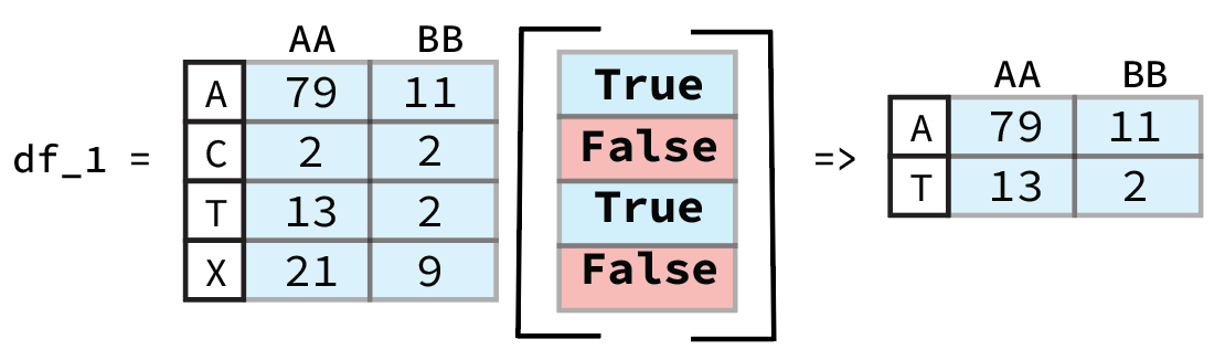
It might seem counterintuitive not to use .loc or .iloc even though we are selecting rows. This is due to the fact that the output of df['press dbar'] < 380 is a Pandas Series that contains information on the row and Pandas inherently assumes that when it is passed a boolean list like this that we want to select those rows that are True. A graphic example of this is shown below.
Sorting
There may also come a time when we want to see the data sorted by some criterion in order to explore potential patterns and order statistics of the entries based on a relation. For example, we might want to order a DataFrame by the depth that a sample was recovered from. Note: We can also sort the order of the columns based on their names.
There are two primary approaches for sorting a DataFrame: one based on the index and the other based on values. When sorting by the index (it’s important to note that the index can represent either row or column labels), you can utilize the sort_index() method. This method accepts an argument for the axis parameter (0 for rows, 1 for columns). In our specific case using DataFrame df, since the rows are already sorted, we can reconfigure the order of the columns instead by specifiying axis=1
Python
df.sort_index(axis=1)
Output
           coxy umol/kg  csal PSS-78  date mmddyy     ph  press dbar  temp ITS-90
Sample ID
Sample-1            NaN      35.0636        40610  7.951       239.8      18.9625
Sample-2          192.3      34.6103        40610    NaN       280.7      16.1095
Sample-3          190.8      34.2475        40610    NaN       320.1      12.9729
Sample-4          191.3      34.1884        40610  7.780       341.3      11.9665
Sample-5          203.5      34.1709        40610    NaN       360.1      11.3636
Sample-6          193.7      34.1083        40610    NaN       385.0      10.4636
Sample-7          156.5      34.0567        40610    NaN       443.7       8.5897
Sample-8          110.7      34.0424        40610  7.496       497.8       7.1464
Here we can see that we’ve ordered the columns alphabetically.
If we want to order the DataFrame based on the value in a particular column or row we instead use sort_values(). We can again use the pressure i.e. ‘press dbar’ column as an example and sort the rows by greatest to smallest pressure value.
Python
df.sort_values(by='press dbar', axis=0, ascending=False)
Will produce the reorder DataFrame as the output:
Output
           date mmddyy  press dbar  temp ITS-90  csal PSS-78  coxy umol/kg     ph
Sample ID
Sample-8         40610       497.8       7.1464      34.0424         110.7  7.496
Sample-7         40610       443.7       8.5897      34.0567         156.5    NaN
Sample-6         40610       385.0      10.4636      34.1083         193.7    NaN
Sample-5         40610       360.1      11.3636      34.1709         203.5    NaN
Sample-4         40610       341.3      11.9665      34.1884         191.3  7.780
Sample-3         40610       320.1      12.9729      34.2475         190.8    NaN
Sample-2         40610       280.7      16.1095      34.6103         192.3    NaN
Sample-1         40610       239.8      18.9625      35.0636           NaN  7.951
Key Points
- Select columns by using
[\"column name\"]or rows by using thelocattribute. - Sort based on values in a column by using the
sort_valuesmethod.
Exercise: Subsetting a Data Set
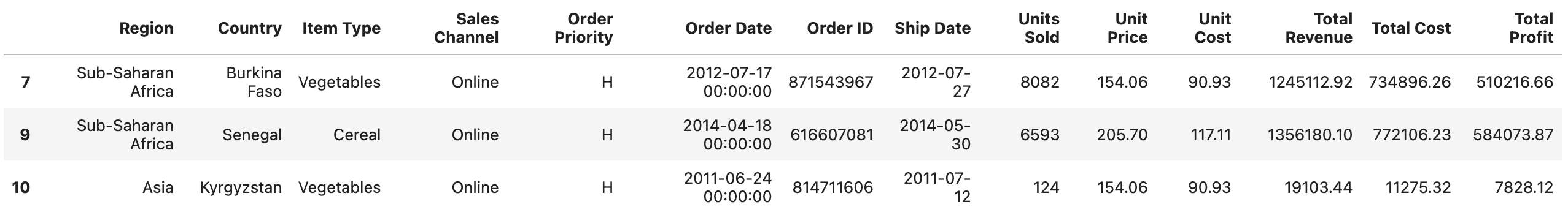
Try it yourself! Going back to our 20_sales_records.xlsx file, identify which orders are Online and High Priority
- Read the first couple rows to get a sense of the data. Which column contains the status (
OnlineorOffline). - A ‘High Priority’ order is indicated by the label ‘H’ in a designated column.
- Retrieve all rows that correspond to online and high-priority orders. In Pandas, you have the option to combine conditions using the
&(and) and|(or) operators, as opposed to Python’s ‘and’ and ‘or’ operators.
Solution
First, we read in the first few lines of our data set to identify which columns we want to filter on. We wantOnline orders of High Priority
  df = pd.read_excel('data/20_sales_records.xlsx', nrows=5)
  df
From the first few rows of data, we see that the column "Sales Channel" describes online/offline status and "Order Priority" describes order priority.
So we use loc along with a combination of conditionals to subset our DataFrame for rows with "Online" entries of "Sales Channel" and "H" level "Order Priority".
df.loc[(df['Sales Channel'] == 'Online') & (df['Order Priority'] == 'H')]The resulting subset should show rows 7, 9, and 10 only. Below is an image that shows how the subsetted `DataFrame` now looks: