Change-HI/EDU (Archive 2022-2023)

This is a time series prediction tutorial using Pytorch. Pytorch is an open source software used in machine learning particularly for training neural networks. This tutorial will use a Pytorch recurrent neural network model to step through the basic workflow of a machine learning project:

Installing Pytorch

Installing deep learning software stacks can be tricky. Pytorch and other deep learning frameworks like Tensorflow and JAX are under rapid development and often depend on particular versions of dependencies.

Google Colab is the easiest way to do the following activity because Pytorch comes preinstalled. Otherwise, use Anaconda to install Pytorch in a new conda environment.

The TsangStreamLab dataset

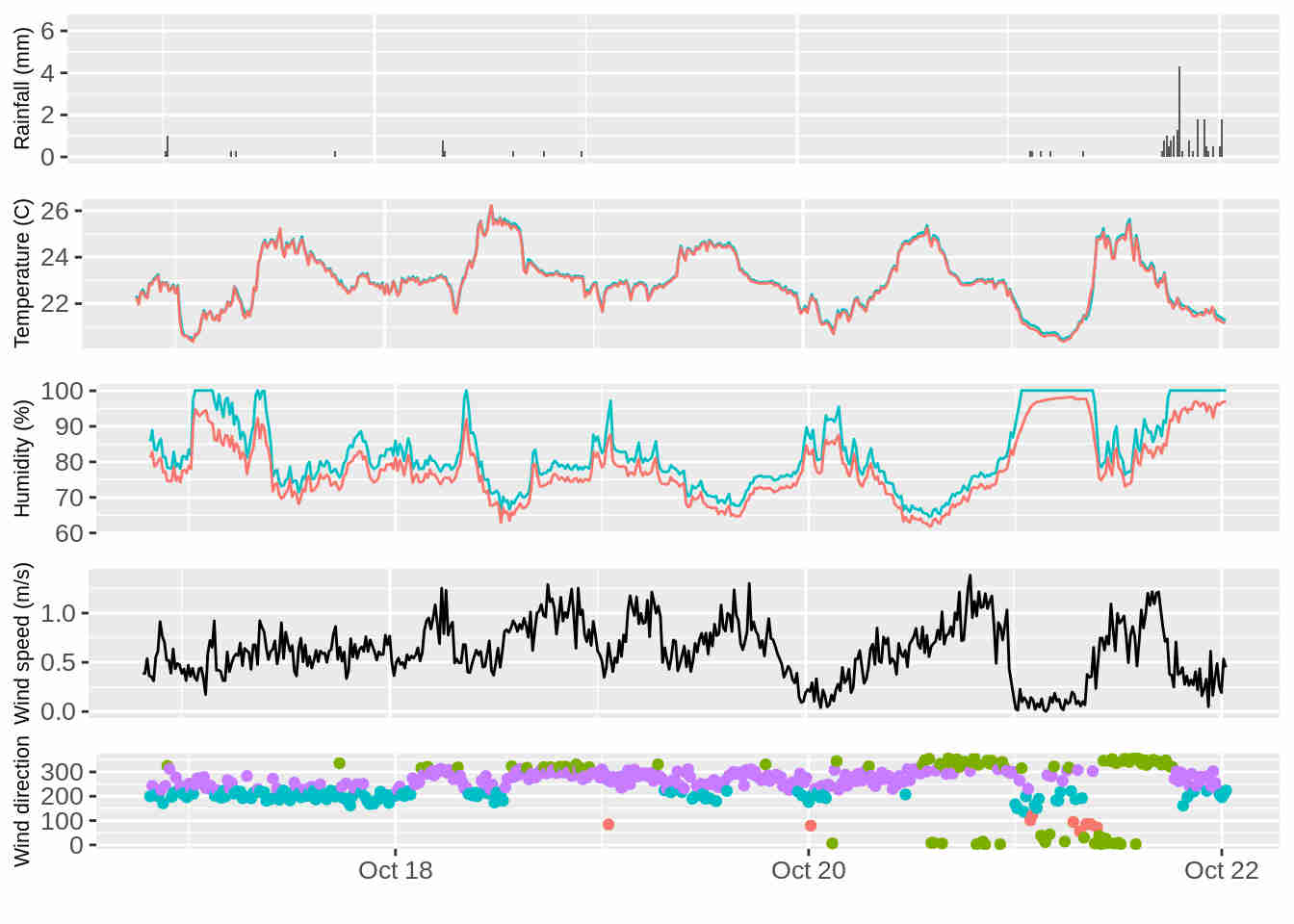
UH Professor Yinphan Tsang’s lab monitors rainfall and stream flow in Manoa Valley. Sensors at Lyon’s arboretum take data at regular 15 minute intervals. Raw data can be downloaded from her website.

A subset of the data has already been downloaded for this workshop. In particular, we will use the pyranometer data which quantifies the amount of solar radiation hitting the ground. We will perform timeseries forecasting with a recurrent neural network. Forecasting solar irradiation is important for managing the variability in renewable energy production.

Activity: Timeseries Model in Pytorch

Exercise: Import dataset, check configuration

Import Libraries

To start, import all the relevant libraries.

import numpy as np
import pandas as pd
import matplotlib.pyplot as plt
from tqdm import tqdm
from sklearn.preprocessing import MinMaxScaler

import torch
import torch.nn as nn
import torch.nn.functional as F
import torch.optim as optim

%matplotlib inline

Download and Preprocess Data

Download the data from this link. This .csv file contains three columns: a timestamp, a measurement of shortwave radiation (in Watts/meter^2) from the sun, and a measurement of rainfall (in mm). Measurements are every 15 minutes from 2018-02-23 12:30:00 to 2020-12-03 12:30:00.

Move or upload the file into your jupyterlab workspace. Load the data into a pandas dataframe.

df = pd.read_csv('./lyons_radiation.csv')

Now let’s preprocess the data. First we set the index of the dataframe to be a series of DateTime objects. This lets pandas know that we are working with timestamps. We then fill in any missing timesteps using the forward fill method, which simply copies previous observations forward to fill any gaps. This is probably not the best method; usually we would inspect the data and use a more careful method, but this is simple, fast, and good enough for this demo.

df['timestamp'] = pd.to_datetime(df['timestamp'])
df = df.set_index(['timestamp'])
df = df.resample('15min').last().ffill()

Now we convert the radiation column into a numpy vector (removing meta data), and scale the values to be between zero and one. Large data values make it much more difficult to train the neural network, so it is critical to make the data (both inputs and outputs) neural network friendly. The Scikit-Learn package has nice tools for doing this. Remember that after training, any model predictions will need to undergo the inverse transform to get useful predictions.

We also convert the timeseries vector into a torch FloatTensor, since that is the data format expected by Pytorch.

data = df['radiation'].to_numpy(dtype='float32')
scaler = MinMaxScaler(feature_range=(0, 1))
data_normalized = scaler.fit_transform(data.reshape(-1, 1))
data_normalized = torch.FloatTensor(data_normalized).view(-1)

Define the Training Set

Training a neural network model is done by presenting sets of (input, output) example pairs. We need to specify what those examples should look like. Our inputs can be of arbitrary length, but we choose to only consider a finite length of 100 timesteps because this is approximately one day (15min * 4 * 24 hrs/day = 1 day).

def create_in_out_pairs(input_data, tw):
    inout_seq = []
    L = len(input_data)
    for i in range(L-tw):
        train_seq = input_data[i:i+tw]
        train_label = input_data[i+tw:i+tw+1]
        inout_seq.append((train_seq ,train_label))
    return inout_seq

train_window = 100
in_out_data = create_in_out_pairs(data_normalized, train_window)

We select a small sample of the total dataset as our training set, leaving some examples for evaluating the model.

train_in_out_data = in_out_data[100:1000:10]

Creating Train/Test Splits

In machine learning, it is critical to split the data into “training” and “test” sets. The training set is used to train the model, while the test set is used to evaluate the model. Machine learning models tend to memorize the training data, so the training error always goes to zero — the only way to know if the model generalizes to new data is by evaluating the performance on the test set, a method known as cross-validation.

In timeseries data, there is a danger of information leakage where the training set is highly correlated to the test set (even if the exact examples are different). Thus, it is common use chrono-cross-validation, where the training data consists of examples before a certain time T, while the test set consists of examples after time T.

Defining the Model

A Long-Short Term Memory (LSTM) neural network is a particular neural network architecture adept at processing sequence data. Because of their recurrent structure, they can take input sequences of arbitrary length (though in practice we limit the length due to computational constraints). See this blog post for a good introduction to recurrent neural networks (RNNs).

Pytorch provides a convenient way to define a complex model in a couple lines of code.

class LSTM(nn.Module):
    def __init__(self, input_size=1, hidden_layer_size=100, output_size=1):
        super().__init__()
        self.hidden_layer_size = hidden_layer_size

        self.lstm = nn.LSTM(input_size, hidden_layer_size)

        self.linear = nn.Linear(hidden_layer_size, output_size)

        self.hidden_cell = (torch.zeros(1,1,self.hidden_layer_size),
                            torch.zeros(1,1,self.hidden_layer_size))

    def forward(self, input_seq):
        lstm_out, self.hidden_cell = self.lstm(input_seq.view(len(input_seq) ,1, -1), self.hidden_cell)
        predictions = self.linear(lstm_out.view(len(input_seq), -1))
        return predictions[-1]
    
model = LSTM(input_size=1, hidden_layer_size=10, output_size=1)

We now have a Pytorch neural network model that takes in a sequence of values, and outputs a prediction (a single scalar). The model parameters have been initialized randomly, so the predictions are random. Now we need to train the model using our dataset.

Designing a neural network architecture

The neural network architecture can have a large impact on performance. The inductive bias of a model refers to the set of assumptions and prior beliefs that are inherent in this choice. All machine learning models have inductive bias. This is not a bad thing, but it means some models are more appropriate for some problems than others. This is formalized in what is known as The No Free Lunch Theorem.

Experienced practicioners know which architectures tend to work best for certain types of problems. Bigger models usually work better, but are slower because of computational constraints. In practice, it is common to try lots of different models and perform model selection to pick the best based on how well the model performs on a test set.

Training the Model

Training the model is an iterative process. Starting from randomly initialized parameters, we iterate through the training examples, make predictions, and update the weight parameters to minimize the loss function. In this case, we use the mean squared error (MSE) loss. We keep track of the average loss over the training set, and report it every time we iterate through the training dataset — each iteration through the training set is called an epoch.

loss_function = nn.MSELoss()
optimizer = torch.optim.Adam(model.parameters(), lr=0.001)
epochs = 20

for i in range(epochs):
    for x, y in train_in_out_data:
        optimizer.zero_grad()
        model.hidden_cell = (torch.zeros(1, 1, model.hidden_layer_size),
                             torch.zeros(1, 1, model.hidden_layer_size))

        y_pred = model(x)

        single_loss = loss_function(y_pred, y)
        single_loss.backward()
        optimizer.step()

    if True: #i%1 == 1:
        print(f'epoch: {i:3} loss: {single_loss.item():10.8f}')

print(f'epoch: {i:3} loss: {single_loss.item():10.10f}')

Solution

epoch:   0 loss: 0.04469438
epoch:   1 loss: 0.04004482
epoch:   2 loss: 0.03381182
epoch:   3 loss: 0.02361814
epoch:   4 loss: 0.01961462
epoch:   5 loss: 0.01725977
epoch:   6 loss: 0.01528491
epoch:   7 loss: 0.01404397
epoch:   8 loss: 0.01311346
epoch:   9 loss: 0.01235864
epoch:  10 loss: 0.01172257
epoch:  11 loss: 0.01118899
epoch:  12 loss: 0.01075610
epoch:  13 loss: 0.01042009
epoch:  14 loss: 0.01016921
epoch:  15 loss: 0.00998601
epoch:  16 loss: 0.00985228
epoch:  17 loss: 0.00975257
epoch:  18 loss: 0.00967518
epoch:  19 loss: 0.00961193
epoch:  19 loss: 0.0096119326

How do I know if it’s working?

Training a neural network is notoriously difficult. The problem is that we are performing stochastic gradient descent optimization on a very non-convex function. You should look to see that the loss function decreases during the first few epochs, indicating that the model is improving. If it doesn’t, try decreasing the learning rate. If that doesn’t help, then you have a bug or the model is not appropriate for your problem.

How long do I train?

It is hard to know when to stop training, because even when the model seems to have converged, it might suddenly have “a revelation” that allows it to explain the training data perfectly. To build your intuition, we highly recommend playing with the toy neural networks in Tensorflow Playground.

In practice, we train until we run out of patience or when we start overfitting to a held out test set (known as early stopping).

Evaluating the Model

Typically we will evaluate the model on a clean, held-out test set that has not been used for training. Evaluation is done by comparing the test set predictions with ground truth labels and computing metrics such as the MSE. Here, we simply demonstrate predictions and visualize them.

The model should be set to eval mode, then we can pass in some test input sequence to get a prediction for the next value. Iteratively passing in the previous input gives a predicted sequence.

test_inputs = data_normalized[-train_window:].tolist()
print(test_inputs)

model.eval()

fut_pred = 12  # Number of predictions to make.
for i in range(fut_pred):
    seq = torch.FloatTensor(test_inputs[-train_window:])
    with torch.no_grad():
        model.hidden = (torch.zeros(1, 1, model.hidden_layer_size),
                        torch.zeros(1, 1, model.hidden_layer_size))
        test_inputs.append(model(seq).item())
        
# Predictions need to be scaled back into W/m^2
actual_predictions = scaler.inverse_transform(np.array(test_inputs[train_window:] ).reshape(-1, 1))

We can plot the observed and predicted values. Pandas datetimes can be used to label the x-axis.

plt.title('')
plt.ylabel('Solar Irradiance $(W/m^2)$')
plt.grid(True)
plt.autoscale(axis='x', tight=True)
plt.plot(data[-train_window:], label='Observed')
plt.plot(np.arange(train_window, train_window +fut_pred), actual_predictions, label='Predicted')
plt.xticks(ticks=np.arange(0, train_window, 20), 
           labels=df['radiation'][-train_window:].index[np.arange(0, 100, 20)], 
           rotation=45)
plt.legend()
plt.show()

Improving the model

If we want to improve the model, the first thing to ask ourselves is whether we are underfitting or overfitting. If we are not overfitting, then we are underfitting and we should increase the size of the model and train longer. If we are overfitting, then we should add regularization or get more training data.

Tutorial of Timeseries Modeling with Deep Learning