Overview

Questions

How can we model environmental data with decision trees?

Objectives

Understand how to fit decision trees in SciKit-Learn

Decision Trees on Mauna Loa CO2 data

This example uses data that consists of the monthly average atmospheric CO2 concentrations (in parts per million by volume (ppm)) collected at the Mauna Loa Observatory in Hawaii, between 1958 and 2001. The objective is to model the CO2 concentration as a function of the time t.

Build the dataset

We will derive a dataset from the Mauna Loa Observatory that collected air samples. We are interested in estimating the concentration of CO2 and extrapolate it for further year. First, we load the original dataset available in OpenML.

from sklearn.datasets import fetch_openml

co2 = fetch_openml(data_id=41187, as_frame=True, parser="pandas")
co2.frame.head()

First, we process the original dataframe to create a date index and select only the CO2 column.

import pandas as pd

co2_data = co2.frame
co2_data["date"] = pd.to_datetime(co2_data[["year", "month", "day"]])
co2_data = co2_data[["date", "co2"]].set_index("date")
co2_data.head()

co2_data.index.min(), co2_data.index.max()

Out: (Timestamp('1958-03-29 00:00:00'), Timestamp('2001-12-29 00:00:00'))

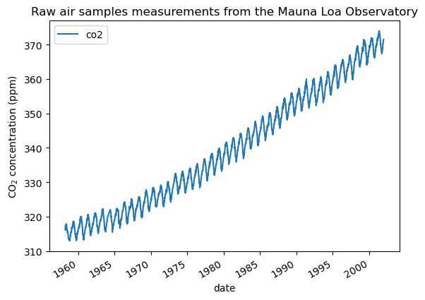
We see that we get CO2 concentration for some days from March, 1958 to December, 2001. We can plot these raw information to have a better understanding.

import matplotlib.pyplot as plt

co2_data.plot()
plt.ylabel("CO$_2$ concentration (ppm)")
_ = plt.title("Raw air samples measurements from the Mauna Loa Observatory")

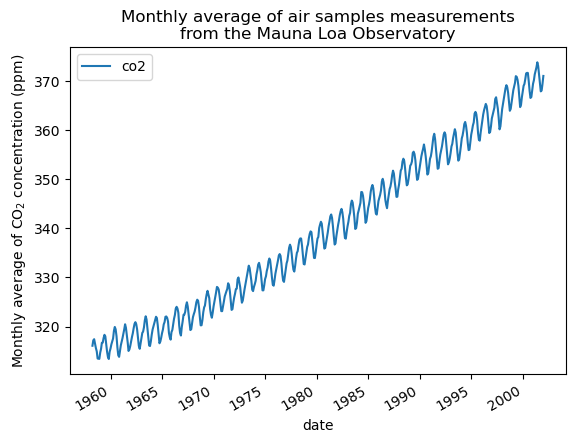
/archive-2022-2023/Basic%20Binder%20Webpage

We will preprocess the dataset by taking a monthly average and drop month for which no measurements were collected. Such a processing will have an smoothing effect on the data.

co2_data = co2_data.resample("M").mean().dropna(axis="index", how="any")
co2_data.plot()
plt.ylabel("Monthly average of CO$_2$ concentration (ppm)")
_ = plt.title(
    "Monthly average of air samples measurements\nfrom the Mauna Loa Observatory"
)

The idea in this example will be to predict the CO2 concentration in function of the date. We are as well interested in extrapolating for upcoming year after 2001.

As a first step, we will divide the data and the target to estimate. The data being a date, we will convert it into a numeric.

X = (co2_data.index.year + co2_data.index.month / 12).to_numpy().reshape(-1, 1)
y = co2_data["co2"].to_numpy()

Model fitting using Decision Tree Regression

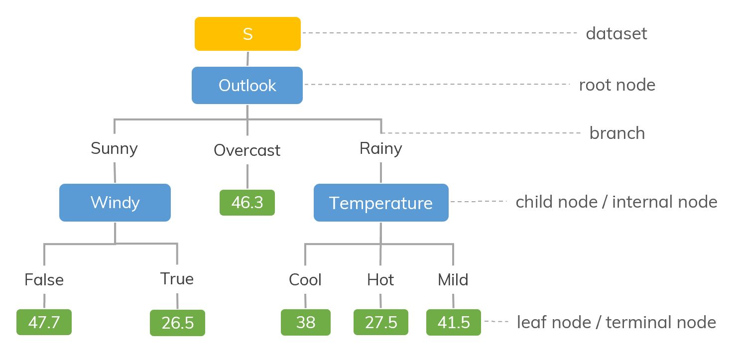
Decision Trees (DTs) are a non-parametric supervised learning method used for classification and regression. The goal is to create a model that predicts the value of a target variable by learning simple decision rules inferred from the data features. A tree can be seen as a piecewise constant approximation.

Decision trees learn from data to approximate a function with a set of if-then-else decision rules. The deeper the tree, the more complex the decision rules. Deeper trees are more powerful, but this can lead to overfitting.

from sklearn import tree
regr_1 = tree.DecisionTreeRegressor(max_depth=2)
regr_2 = tree.DecisionTreeRegressor(max_depth=11)
regr_1.fit(X, y)
regr_2.fit(X, y)

Now, we will use the the fitted models to predict on:

training data to inspect the goodness of fit;

future data to see the extrapolation done by the models.

Thus, we create synthetic data from 1958 to the current month.

import datetime
import numpy as np

today = datetime.datetime.now()
current_month = today.year + today.month / 12
X_test = np.linspace(start=1958, stop=current_month, num=1_000).reshape(-1, 1)

y_1 = regr_1.predict(X_test)
y_2 = regr_2.predict(X_test)

plt.figure()
plt.scatter(X, y, s=20, edgecolor="black", c="darkorange", label="data")
plt.plot(X_test, y_1, color="cornflowerblue", label=f"max_depth={regr_1.max_depth}", linewidth=2)
plt.plot(X_test, y_2, color="yellowgreen", label=f"max_depth={regr_2.max_depth}", linewidth=2)
plt.xlabel("data")
plt.ylabel("target")
plt.title("Decision Tree Regression")
plt.legend()
plt.show()

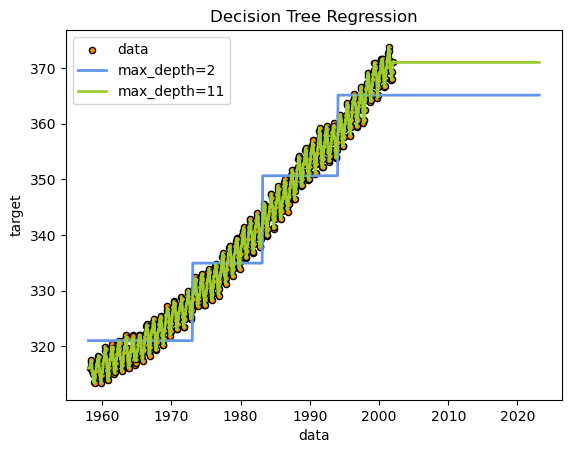
As you can see, the decision tree regression was able to fit data within the existing domain quite well. The criteria for decisions is intuitive and can be understood with a simple visualization. However, it has completely failed to predict any future trend outside the domain it was trained on.

Model the derivative of the data

To improve the model’s generalization, we will predict on differences in CO2 rather than absolute CO2 levels, using a “sliding window” of recent CO2 differences as the input. We will also normalize the data.

from sklearn.preprocessing import StandardScaler
from numpy import diff

def preprocess_data(input_data, train_window):
    # Take derivative
    input_data = np.concatenate([[0], diff(input_data)])
    
    # Scale values
    scaler = StandardScaler()
    normalized_data = scaler.fit_transform(input_data.reshape(-1, 1)).reshape(-1)
    
    # Create input-output pairs
    in_seq = []
    out_seq = []
    L = len(normalized_data)
    for i in range(L-train_window-1):
        train_seq = normalized_data[i:i+train_window]
        train_label = normalized_data[i+train_window:i+train_window+1]
        
        in_seq.append(train_seq)
        out_seq.append(train_label)
    return normalized_data, in_seq, out_seq, scaler

train_window = 50
normalized_data, in_data, out_data, scaler = preprocess_data(list(co2_data["co2"]), train_window)

We will train 3 decision trees at different max depths.

regr_3 = tree.DecisionTreeRegressor(max_depth=2)
regr_3.fit(in_data, out_data)

regr_4 = tree.DecisionTreeRegressor(max_depth=10)
regr_4.fit(in_data, out_data)

regr_5 = tree.DecisionTreeRegressor(max_depth=25)
regr_5.fit(in_data, out_data)

Now we will generate test data that runs all the way to the present day to see the model’s predictions. We use the model’s own prediction as part of the sliding window for the next prediction, to extrapolate arbitrarily far into the future.

dates = pd.period_range("1958", "2023", freq='M').to_timestamp()


test_inputs = list(normalized_data)
fut_pred_3 = test_inputs.copy()
fut_pred_4 = test_inputs.copy()
fut_pred_5 = test_inputs.copy()
fut_pred_num = len(dates) - len(test_inputs)  # Number of predictions to make.
for i in range(fut_pred_num):
    seq = fut_pred_3[-train_window:]
    prediction = regr_3.predict([seq])
    fut_pred_3.append(prediction[0])
    
    seq = fut_pred_4[-train_window:]
    prediction = regr_4.predict([seq])
    fut_pred_4.append(prediction[0])
    
    seq = fut_pred_5[-train_window:]
    prediction = regr_5.predict([seq])
    fut_pred_5.append(prediction[0])

Let’s plot the results. Note that it is still showing the differences (derivative) rather than the absolute value, and it’s still normalized.

plt.figure()
plt.plot(dates, fut_pred_3, label=f"max_depth={regr_3.max_depth}", linewidth=2)
plt.plot(dates, fut_pred_4, label=f"max_depth={regr_4.max_depth}", linewidth=2)
plt.plot(dates, fut_pred_5, label=f"max_depth={regr_5.max_depth}", linewidth=2)
plt.plot(dates[0:526], normalized_data, label=f"true value", linewidth=2)
plt.xlabel("data")
plt.ylabel("target")
plt.title("Decision Tree Regression on Derivative")
plt.legend()
plt.show()

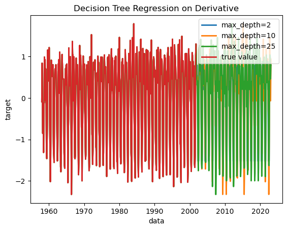
We can see that all of the decision trees are fitting the past data nearly perfectly, but do not entirely agree on future predictions.

Let’s convert the predictions back into absolute CO2 levels.

def postprocess_data(output_data, scaler, first_input):
    #unscale the output
    output = scaler.inverse_transform(np.array(output_data).reshape(-1, 1)).reshape(-1)
    
    output = np.cumsum(output) + first_input
    
    return output

decoded_3 = postprocess_data(fut_pred_3, scaler, list(co2_data["co2"])[0])
decoded_4 = postprocess_data(fut_pred_4, scaler, list(co2_data["co2"])[0])
decoded_5 = postprocess_data(fut_pred_5, scaler, list(co2_data["co2"])[0])

And plot the results:

plt.figure()
plt.plot(dates, decoded_3, label=f"max_depth={regr_3.max_depth}", linewidth=2)
plt.plot(dates, decoded_4, label=f"max_depth={regr_4.max_depth}", linewidth=2)
plt.plot(dates, decoded_5, label=f"max_depth={regr_5.max_depth}", linewidth=2)
plt.xlabel("data")
plt.ylabel("target")
plt.title("Decision Tree Regression")
plt.legend()
plt.show()

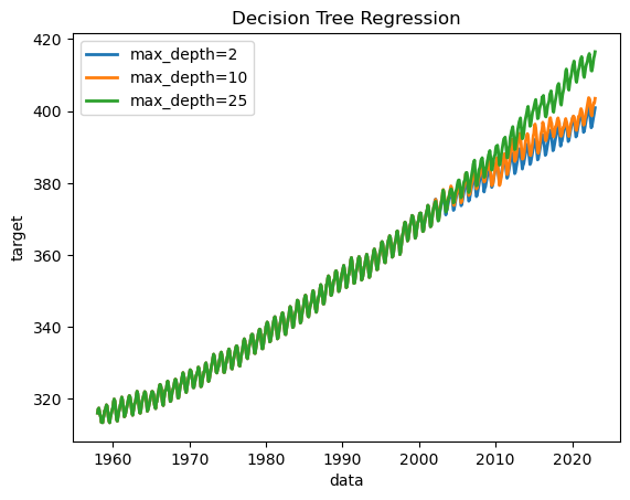
The results can vary quite a bit between runs. The method for fitting the decision trees is stochastic, and our many input variables are all similarly informative, so the tree’s hierarchy can vary significantly. Decision trees are not robust, so slight changes in input or in the tree structure can drastically alter predictions.

For more information

Attribution:

This workshop was modified from the following:

Gaussian process regression (GPR) on Mauna Loa CO2 data

Rasmussen, Carl Edward. “Gaussian processes in machine learning.” Summer school on machine learning. Springer, Berlin, Heidelberg, 2003.

Authors:

Jan Hendrik Metzen jhm@informatik.uni-bremen.de
Guillaume Lemaitre g.lemaitre58@gmail.com

License: BSD 3 clause

SciKit-Learn Decision Tree Regression tutorial SciKit-Learn Decision Tree tutorial