Change-HI/EDU (Archive 2022-2023) | 5. Deep learning CPU vs GPU

Overview

Questions

How does the performance of GPU compare with that of CPU?
How to use Mana to do Machine Learning research?

Objectives

Do a basic Deep Learning tutorial on Mana

Deep Learning Tutorial

This is a basic image classification tutorial from CIFAR-10 dataset using TensorFlow.

About TensorFlow

TensorFlow is an open source software used in machine learning particularly for training neural networks.

We’ll define our model using ‘Keras’- a high level API which acts as an interface between TensorFlow and Python and makes it easy to build and train models. You can read more about it here.

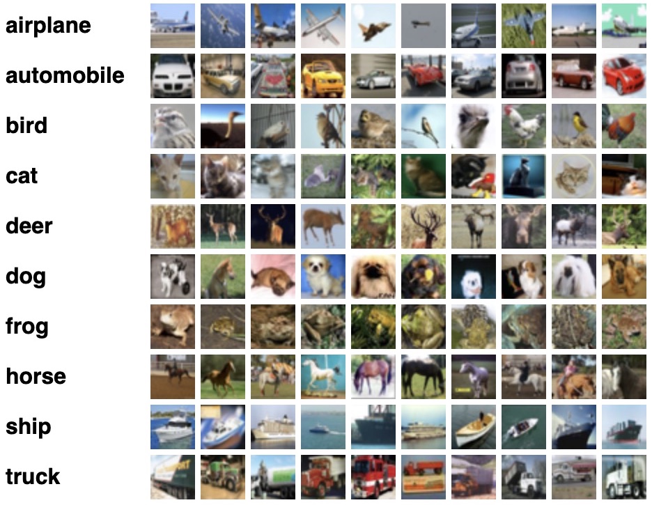
The CIFAR-10 dataset

CIFAR-10 is a common dataset used for machine learning and computer vision research. It is a subset of 80 million tiny image dataset and consists of 60,000 images. The images are labelled with 10 different classes. So each class has 5000 training images and 1000 test images. Each row represents a color image of 32 x 32 pixels with 3 channels (RGB).

Basic workflow of Machine Learning

Collect the data
Pre-process the data
Define a model
Train the model
Evaluate/test the model
Improve your model

Activity: Work with CIFAR-10 dataset

Exercise: Import dataset, check configuration

To start, import all the relevant libraries:

import numpy as np
import matplotlib.pyplot as plt

import tensorflow as tf
import h5py
import keras
from keras.datasets import cifar10
from tensorflow.keras.models import Sequential
from tensorflow.keras.layers import Dense, Conv2D, Flatten, MaxPooling2D, Input, InputLayer, Dropout
import keras.layers.merge as merge
from keras.layers.merge import Concatenate
from tensorflow.keras.utils import to_categorical
from tensorflow.keras.optimizers import SGD, Adam

%matplotlib inline

Next, check to see if you’re using the GPU:

tf.config.list_physical_devices('GPU')

Now, how would you check to see if you’re using the CPU rather than the GPU?

Solution

tf.config.list_physical_devices('CPU')

Is GPU necessary for machine learning?

No, machine learning algorithms can be deployed using CPU or GPU, depending on the applications. They both have their distinct properties and which one would be best for your application depends on factors like: speed, power usage and cost.

CPUs are more general purposed processors, are cheaper and provide a gateway for data to travel from source to GPU cores.

But GPU have an advantage to do parallel computing when dealing with large datasets, complex neural network models. The difference between the two lies in basic features of a processor i.e. cache, clock speed, power consumption, bandwidth and number of cores.

Read more that here.

Exercise: Load the data and analyze its shape

(x_train, y_train), (x_valid, y_valid) = cifar10.load_data()
nb_classes = 10
class_names = ['airplane', 'automobile', 'bird', 'cat', 'deer', 'dog', 'frog', 'horse', 'ship', 'truck']
print('Train: X=%s, y=%s' % (x_train.shape, y_train.shape))
print('Test: X=%s, y=%s' % (x_valid.shape, y_valid.shape))
print('number of classes= %s' %len(set(y_train.flatten())))
print(type(x_train))

Solution

Train: X=(50000, 32, 32, 3), y=(50000, 1)
Test: X=(10000, 32, 32, 3), y=(10000, 1)
number of classes= 10
<class 'numpy.ndarray'>

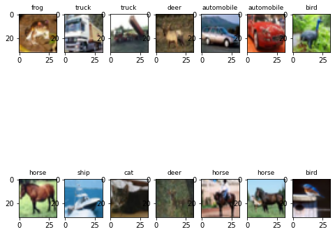
Plot some examples

plt.figure(figsize=(8, 8)) 
for i in range(2*7):
    # define subplot
    plt.subplot(2, 7, i+1)
    plt.imshow(x_train [i])
    class_index = np.argmax(to_categorical(y_train[i], 10))
    plt.title(class_names[class_index], fontsize=9)

Solution

Exercise: Convert data to HDF5 format

with h5py.File('dataset_cifar10.hdf5', 'w') as hf:
    dset_x_train = hf.create_dataset('x_train', data=x_train, shape=(50000, 32, 32, 3), compression='gzip', chunks=True)
    dset_y_train = hf.create_dataset('y_train', data=y_train, shape=(50000, 1), compression='gzip', chunks=True)
    dset_x_test = hf.create_dataset('x_valid', data=x_valid, shape=(10000, 32, 32, 3), compression='gzip', chunks=True)
    dset_y_test = hf.create_dataset('y_valid', data=y_valid, shape=(10000, 1), compression='gzip', chunks=True)

What is an HDF5 file?

HDF5 file format is a binary data format which is mainly used to store large, heterogenous files. It provides fast, parallel I/O processing.

You can learn more about it here and here.

Exercise: Define the model

model = tf.keras.Sequential()
model.add(InputLayer(input_shape=[32, 32, 3]))

model.add(Conv2D(filters=32, kernel_size=3, padding='same', activation='relu'))
model.add(MaxPooling2D(pool_size=[2,2], strides=[2, 2], padding='same'))

model.add(Conv2D(filters=64, kernel_size=3, padding='same', activation='relu'))
model.add(MaxPooling2D(pool_size=[2,2], strides=[2, 2], padding='same'))

model.add(Conv2D(filters=128, kernel_size=3, padding='same', activation='relu'))
model.add(MaxPooling2D(pool_size=[2,2], strides=[2, 2], padding='same'))

model.add(Conv2D(filters=256, kernel_size=3, padding='same', activation='relu'))
model.add(MaxPooling2D(pool_size=[2,2], strides=[2, 2], padding='same'))

model.add(Flatten())

model.add(Dense(256, activation='relu'))
model.add(Dropout(0.2))

model.add(Dense(512, activation='relu'))
model.add(Dropout(0.2))

model.add(Dense(10, activation='softmax'))

model.summary()

Exercise: Define the data generator

class DataGenerator(tf.keras.utils.Sequence):
   
    def __init__(self, batch_size, test=False, shuffle=True):      
        PATH_TO_FILE = 'dataset_cifar10.hdf5'       
        self.hf = h5py.File(PATH_TO_FILE, 'r')         
        self.batch_size = batch_size
        self.test = test
        self.shuffle = shuffle
        self.on_epoch_end()

    def __del__(self):
        self.hf.close()
       
    def __len__(self):
        return int(np.ceil(len(self.indices) / self.batch_size))

    def __getitem__(self, idx):
        start = self.batch_size * idx
        stop = self.batch_size * (idx+1)       
        if self.test:
            x = self.hf['x_valid'][start:stop, ...]
            batch_x = np.array(x).astype('float32') / 255.0
            y = self.hf['y_valid'][start:stop]
            batch_y = to_categorical(np.array(y), 10)
        else:
            x = self.hf['x_train'][start:stop, ...]
            batch_x = np.array(x).astype('float32') / 255.0
            y = self.hf['y_train'][start:stop]
            batch_y = to_categorical(np.array(y), 10)
        return batch_x, batch_y

    def on_epoch_end(self):
        if self.test:
            self.indices = np.arange(self.hf['x_valid'][:].shape[0])
        else:
            self.indices = np.arange(self.hf['x_train'][:].shape[0])          
        if self.shuffle:
            np.random.shuffle(self.indices)

Exercise: Generate batches of data for training and validation dataset

batchsize  = 250 
data_train = DataGenerator(batch_size=batchsize)
data_valid = DataGenerator(batch_size=batchsize, test=True, shuffle=False)

Exercise: First, let’s train the model using CPU

 with tf.device('/device:CPU:0'):
    history = model.fit(data_train,epochs=10, verbose=1, validation_data=data_valid)

Exercise: Now, let’s compare GPU to CPU performance.

First, let’s get the CPU performance data.

from tensorflow.keras.models import clone_model
new_model = clone_model(model)
opt = keras.optimizers.Adam(learning_rate=0.001)
new_model.compile(optimizer=opt, loss='categorical_crossentropy', metrics=['accuracy'])  

Exercise: Train the new model with GPU

Can you do this yourself?

Solution

with tf.device('/device:GPU:0'):
  new_history = new_model.fit(data_train,epochs=10, verbose=1, validation_data=data_valid)

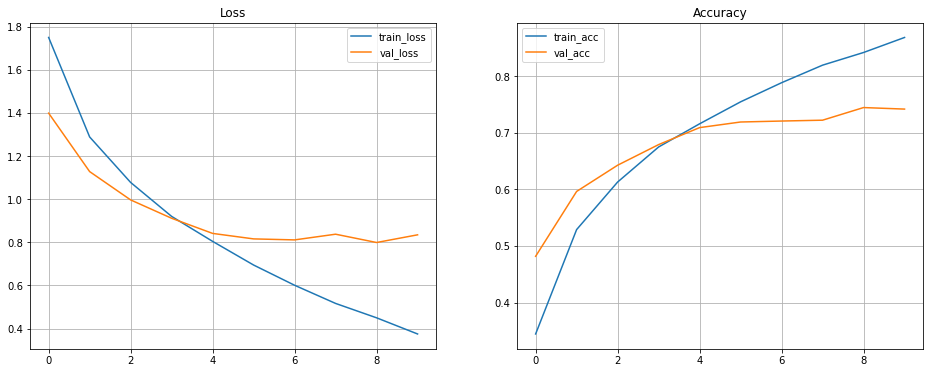
Exercise: Plot the losses and accuracy for training and validation set

fig, axes = plt.subplots(1,2, figsize=[16, 6])
axes[0].plot(history.history['loss'], label='train_loss')
axes[0].plot(history.history['val_loss'], label='val_loss')
axes[0].set_title('Loss')
axes[0].legend()
axes[0].grid()
axes[1].plot(history.history['accuracy'], label='train_acc')
axes[1].plot(history.history['val_accuracy'], label='val_acc')
axes[1].set_title('Accuracy')
axes[1].legend()
axes[1].grid()

Solution

Exercise: Evaluate the model and make predictions

x = x_valid.astype('float32') / 255.0
y = to_categorical(y_valid, 10)
score = new_model.evaluate(x, y, verbose=0)
print('Test cross-entropy loss: %0.5f' % score[0])
print('Test accuracy: %0.2f' % score[1])

y_pred = new_model.predict_classes(x)

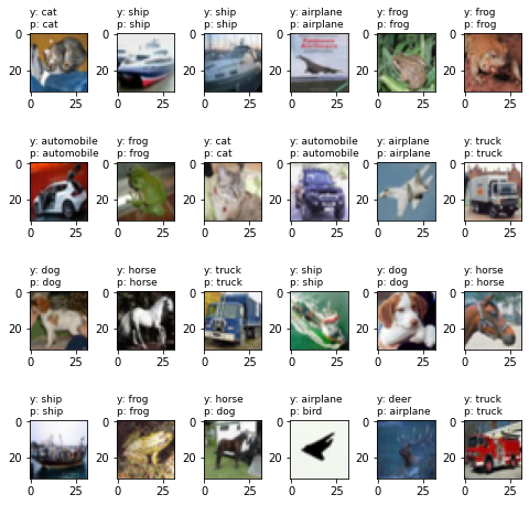
Exercise: Plot the predictions

plt.figure(figsize=(8, 8)) 
for i in range(20):
    plt.subplot(4, 5, i+1)
    plt.imshow(x[i].reshape(32,32,3))
    index1 = np.argmax(y[i])
    plt.title("y: %s\np: %s" % (class_names[index1], class_names[y_pred[i]]), fontsize=9, loc='left')
    plt.subplots_adjust(wspace=0.5, hspace=0.4)

Solution

Other Machine Learning resources

You can use Google Colab which uses Jupyter notebooks too but on Google server. Here you can get free limited compute resources (even GPU) and upgrade your account (for TPU) if you want more. The code usually runs on Google servers on cloud and is connected to your google account so all your projects will be saved in your Google Drive.
Microsoft Azure notebook is similar to Google Colab with cloud sharing functionality but provides more memory.
Kaggle
Amazon Sage Maker

Discussion: Why HPC?

Why would you need an HPC cluster over your personal computer?

Key Points

Open On Demand requires you have a strong, stable internet connection whereas SSH can work with weak connections too.
JupyterLab is a more common platform for data science research but there are other IDE (Integrated Development Environment softwares) like PyCharm, Spyder, RMarkdown too.
Using multiple GPUs won’t improve the performance of your machine learning model. It only helps for a very complex computation or large models.