4. Wrangling DataFrames
Overview
Questions
- How can you select individual columns or rows from a
DataFrame? - How can you subset a
DataFrame? - How can you sort a
DataFrame?
Objectives
- Learn how to select specific columns or rows from a
DataFrame - Learn how to select rows based on conditions.
- Learn how to sort a
DataFrame’s rows or columns.
![]()
Selection, Subsetting and Sorting a DataFrame
When exploring our data we will often want to focus our attention to specific rows, columns, and entries that satisfy certain conditions. We may want to either look at a single column of the data or work with a subset of the original data. This situation may occur because the source of your data was probably not using the information for the exact same purpose.
Furthermore, it is often helpful to sort our data set using a particular relation to identify patterns and to understand the data’s structure. For example, suppose the original data set we acquire and want to analyze describes a sport team’s performance for each game during a season and it is original ordered in chronological order. It may be interesting to sort the game play statistics using a different relation such as number of points scored to easily identify high and low scoring games.
As with previous episodes you should follow along in the notebook starting with ‘04’ that can be found at the following link Link to Binder.
Selection
Selecting data from a DataFrame is very easy and builds on concepts we discussed in the previous episode. As mentioned previously, in a DataFrame we have column names called headers and row names called indexes. Depending on how we loaded the data these might be integers or some other ID.
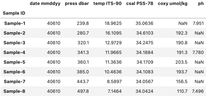
If we have the example DataFrame seen in the image below we can select and/or subset various combinations of rows and columns by using Pandas.
Selecting Columns
To start off lets focus on subsetting columns. If we have a DataFrame called df and a column called ‘ph’ we can subset the DataFrame using df['ph'].
Python
df['ph']
Output
Sample ID
Sample-1    7.951
Sample-2      NaN
Sample-3      NaN
Sample-4    7.780
Sample-5      NaN
Sample-6      NaN
Sample-7      NaN
Sample-8    7.496
Name: ph, dtype: float64
Selecting Rows
If on the other hand we want to access a subset rows we have to use a slightly different approach. While previously we could just pass the name of the column inside brackets if we want to access one or more rows we need to use the .loc or .iloc methods.
So if we again have a DataFrame called df and a row called ‘Sample-1’ we can access it using df.loc['Sample-1', df.columns].
Python
df.loc['Sample-1', df.columns]
Output
date mmddyy     40610.0000
press dbar        239.8000
temp ITS-90        18.9625
csal PSS-78        35.0636
coxy umol/kg           NaN
ph                  7.9510
Name: Sample-1, dtype: float64
The key difference between .loc and .iloc is that .loc relies on the names of the indexes and headers while .iloc relies instead on the index and header number. Here df.columns is providing the all the header names in the DataFrame called df and letting pandas know that we want a single row, but all of the header in the DataFrame.
If we were to use .iloc instead of .loc for the previous example and we know that ‘Sample-1’ is at index position 0 we would use df.iloc[0, :] and get the same result. You might notice that we also had to change df.columns to : when we used .iloc this is because df.columns provides the names of all the headers which is fine to do with .loc but not .iloc.
Python
df.iloc[0, :]
Output
date mmddyy     40610.0000
press dbar        239.8000
temp ITS-90        18.9625
csal PSS-78        35.0636
coxy umol/kg           NaN
ph                  7.9510
Name: Sample-1, dtype: float64
The : operator
When used inside a bracket the : operator will return the range between the two values it is given. For example if we had a Python list x with the following values [‘a’, ‘b’, ‘c’, ‘d’, ‘e’] and wanted to select ‘b’, ‘c’, and ‘d’ we can do this very concisely using the : operator.
Python
x = ['a', 'b', 'c', 'd', 'e']
x[2:5]
With the output:
['b', 'c', 'd']
Selecting Columns and Rows Simultaneously
As we saw in the previous section we can select one or more rows and/or columns to view. For example if we wanted to view the ‘ph’ entry of ‘Sample-1’ from the previous example we could use .loc in the following manner.
Python
df.loc['Sample-1', 'ph']
Output
7.951
If we wanted to select multiple columns e.g. both the ‘ph’ and ‘Longitude’ columns we can change the code bit to fit our needs.
Python
df.loc['Sample-1', ['ph', 'Longitude']]
Output
temp ITS-90    18.9625
ph              7.9510
Name: Sample-1, dtype: float64
Using .iloc
You can just as well use .iloc for the two examples above, but you will need to change the index and headers to their respective integer values i.e. the row number(s) and the header number(s).
Subsetting
Comparison operations (“<” , “>” , “==” , “>=” , “<=” , “!=”) can be applied to pandas Series and DataFrames in the same vectorized fashion as arithmetic operations except the returned object is a Series or DataFrame of booleans (either True or False).
Within a Single DataFrame
To start let focus on a single DataFrame to better understand how comparison operations work in Pandas. As an example lets say that we have a DataFrame like the one below stored in df:
If we wanted to identify which of the above samples come from a depth above 380 we start by finding column ‘press dbar’ using a less than condition of 380.
Python
df['press dbar'] < 380
The output will be a Pandas Series containing a boolean value for each row in the df that looks like this.
Output
Sample ID
Sample-1     True
Sample-2     True
Sample-3     True
Sample-4     True
Sample-5     True
Sample-6    False
Sample-7    False
Sample-8    False
Name: press dbar, dtype: bool
We can see that the first row and the last row are both True while the remaining rows are False and a quick look at the original data confirms that this is correct based on our condition. However, looking back at the original DataFrame is very tedious. If we instead want to view/save the rows that were found to have a depth < 380 we can either save the output Series to a variable and use that or directly place the previously used code within a bracket. Both methods are equivalent and shown below.
Python
good_rows = df['press dbar'] < 380
df[good_rows]
Is equivalent to:
Python
df[df['press dbar'] < 380]
Either of these code bits will generate the same output:
Output
           date mmddyy  press dbar  temp ITS-90  csal PSS-78  coxy umol/kg     ph
Sample ID
Sample-1         40610       239.8      18.9625      35.0636           NaN  7.951
Sample-2         40610       280.7      16.1095      34.6103         192.3    NaN
Sample-3         40610       320.1      12.9729      34.2475         190.8    NaN
Sample-4         40610       341.3      11.9665      34.1884         191.3  7.780
Sample-5         40610       360.1      11.3636      34.1709         203.5    NaN
It might seem strange that we don’t need to use .loc or .iloc despite the fact that we are selecting rows. This is due to the fact that the output of df['press dbar'] < 380 is a Pandas Series that contains information on the row and Pandas inherently assumes that when it is passed a boolean list like this that we want to select those rows that are True. A graphic example of this is shown below.
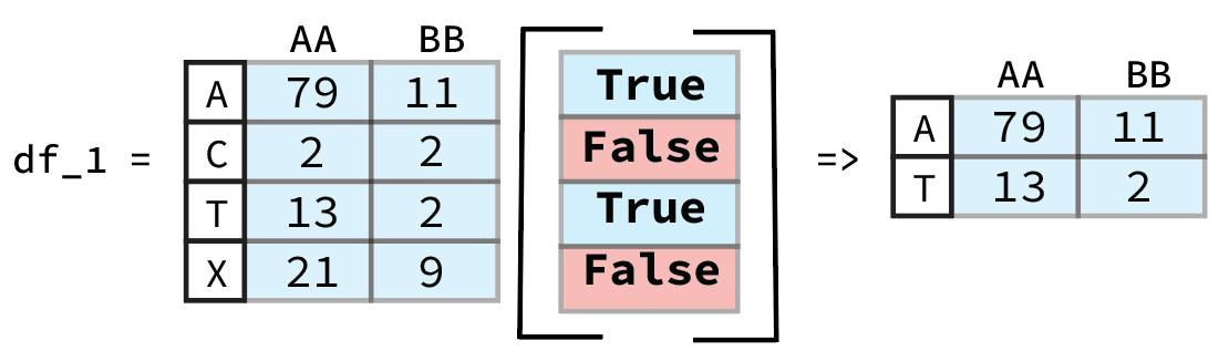
From previous Pandas Data Wrangling workshop (Link to Github).
Column Specification
If you do not specify a column to compare and instead do e.g. df.loc[:] < df2.loc[:] you will get a comparison of every column and a DataFrame containing those values as an output:
Python
df.loc[:] < df2.loc[:]
Output
           date mmddyy  press dbar  temp ITS-90  csal PSS-78  coxy umol/kg     ph
Sample ID
Sample-1          True       False         True         True         False  False
Sample-2          True       False         True         True          True  False
Sample-3          True       False         True         True          True  False
Sample-4          True       False         True         True          True   True
Sample-5          True       False         True         True         False  False
Sample-6          True       False         True         True          True  False
Sample-7          True       False         True         True          True  False
Sample-8          True       False         True         True          True  False
Sorting
There may also come a time when we want to see the data sorted by some criterion in order to explore potential patterns and order statistics of the entries based on a relation. For example, we might want to order a DataFrame by the depth that a sample was recovered from. Note: we can also sort the order of the columns based on their names
There are two primary methods to sort a DataFrame either by the index or by a value. The index is rather straight forward, you use the method sort_index() to sort the DataFrame and provide an axis (0=row, 1=columns). We can reuse df and since the index is already sorted we can sort the order of the columns instead.
Python
df.sort_index(axis=1)
Output
           coxy umol/kg  csal PSS-78  date mmddyy     ph  press dbar  temp ITS-90
Sample ID
Sample-1            NaN      35.0636        40610  7.951       239.8      18.9625
Sample-2          192.3      34.6103        40610    NaN       280.7      16.1095
Sample-3          190.8      34.2475        40610    NaN       320.1      12.9729
Sample-4          191.3      34.1884        40610  7.780       341.3      11.9665
Sample-5          203.5      34.1709        40610    NaN       360.1      11.3636
Sample-6          193.7      34.1083        40610    NaN       385.0      10.4636
Sample-7          156.5      34.0567        40610    NaN       443.7       8.5897
Sample-8          110.7      34.0424        40610  7.496       497.8       7.1464
Here we can see that we’ve ordered the columns alphabetically.
If we want to instead order the DataFrame based on the value in a particular column or row we instead use sort_values(). We can again use the pressure i.e. ‘press dbar’ column as an example and sort the rows by greatest to smallest pressure value.
Python
df.sort_values(by='press dbar', axis=0, ascending=False)
Will produce the reorder DataFrame as the output:
Output
           date mmddyy  press dbar  temp ITS-90  csal PSS-78  coxy umol/kg     ph
Sample ID
Sample-8         40610       497.8       7.1464      34.0424         110.7  7.496
Sample-7         40610       443.7       8.5897      34.0567         156.5    NaN
Sample-6         40610       385.0      10.4636      34.1083         193.7    NaN
Sample-5         40610       360.1      11.3636      34.1709         203.5    NaN
Sample-4         40610       341.3      11.9665      34.1884         191.3  7.780
Sample-3         40610       320.1      12.9729      34.2475         190.8    NaN
Sample-2         40610       280.7      16.1095      34.6103         192.3    NaN
Sample-1         40610       239.8      18.9625      35.0636           NaN  7.951
Key Points
- Select columns by using
[\"column name\"]or rows by using thelocattribute. - Sort based on values in a column by using the
sort_valuesmethod.
Exercise: Subsetting a Data Set
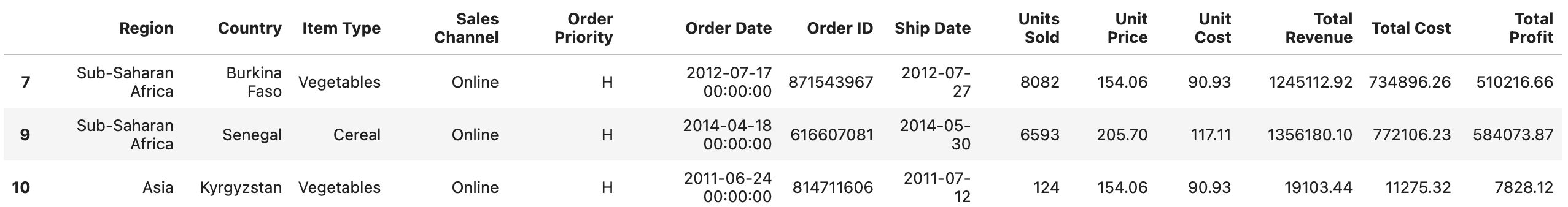
Try it yourself! Going back to our 20_sales_records.xlsx file, idenitfy which orders are Online and High Priority
- Read the first couple rows to get a sense of the data. Which column reflects
OnlineorOfflineStatus. - A
High Priorityorder is denoted byHin one of the columns. Identify which column. - HINT: Use the loc method
Solution
First, we read in the first few lines of our data set to identify which columns we want to filter on. We want `Online` orders of `High Priority`
  df = pd.read_excel('data/20_sales_records.xlsx', nrows=5)
  df
From the first few rows of data, we see that the column "Sales Channel" describes online/offline status and "Order Priority" describes order priority.
So we use loc along with a combination of conditionals to subset our DataFrame for rows with "Online" entries of "Sales Channel" and "H" level "Order Priority".
df.loc[(df['Sales Channel'] == 'Online') & (df['Order Priority'] == 'H')]The resulting subset should show rows 7, 9, and 10 only. Below shows how our subsetted `DataFrame` now looks: